Dissecting UMAP visualizations

In this blog post I aim to showcase the Uniform Manifold Approximation and Projection (UMAP) algorithm from a practical standpoint by experimenting with its various hyperparameters in a single cell RNA-seq (scRNA-seq) dataset of 3,000 cells uniformly sampled from a mouse brain dataset. UMAP is an unsupervised learning algorithm for constructing low-dimensional manifolds in high-dimensional datasets, and is commonly applied for the purpose of data visualization. UMAP and other dimensionality reduction techniques help with interpretability of complex datasets. For example, in the case of scRNA-seq analysis, UMAP helps us understand the differences and similarities between different cells by reducing their transcriptomes from ~20k+ dimensions down to two dimensions that we can inspect visually. Scanpy offets a nice tutorial for getting started with scRNA-seq analysis, including a dataset of peripheral mononuclear blood cells (PBMCs).

In their 2018 arXiv paper, McInnes & Healy introduce UMAP and argue that it is competitive with t-distributed Stochastic Neighbor Embedding (t-SNE) in terms of visualization quality while offering superior run time performance. Additionally, the authors argue that the global structure of the data is better preserved in UMAP compared to t-SNE.

While UMAP can be used for general-purpose dimensionality reduction, in single-cell genomics field it is usually applied to data that has already been reduced using a linear transformation such as principal component analysis (PCA). UMAP has been integrated in almost every single-cell data analysis toolkit, including Seurat and Scanpy.

What does a UMAP plot look like?

The following scatter plot shows the dataset of 3,000 cells and 19,998 genes that has been reduced to 3,000 cells (dots) and 2 UMAP dimensions, visualized in the plot below. Each cell is colored by cluster assignment from Leiden clustering on the PCA reduced dataset.

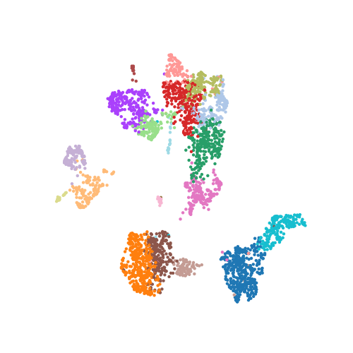
In practice, computing a UMAP with Scanpy is very easy, and you don’t necessarily need to think about hyperparameters at all. The following line of code constructed the above UMAP on the scRNA-seq dataset.

sc.tl.umap(adata)

In many cases it is okay to use UMAP’s default parameters, but if you are like me you may be curious what these default settings are and how they are influencing your interpretation of the data. For single-cell analysis, cells should group together in UMAP space based on cell type identity. Cell types must be carefully annotated by inspecting the distribution of gene expression values in literature curated lists of canonical cell type marker genes, and by using statistical tests to identify up- and down-regulated genes in each cell population. UMAP visualizations of these genes can be helpful to diagnose problematic data processing or erroneous cell type annotations.

Playing with UMAP hyperparameters

Here I show the results of testing different values for seven different UMAP hyperparameters. The following hyperparameter descriptions are taken from the Scanpy documentation.

• n_neighbors: A value between 2 and 100, representing the number of neighboring data points used for manifld approximation. Larger values give a manifold with a more global view of the dataset, while smaller values preserve more of the local structures.
• min_dist: The minimum distance between two points in the UMAP embedding.
• spread: A scaling factor for distance between embedded points.
• gamma: Weighting applied to negative samples in low dimensional embedding optimization.
• alpha: The initial learning rate for UMAP optimization.
• maxiter: The number of iterations for UMAP optimization.
• negative_sample_rate: The number of negative edge/1-simplex samples to use per positive edge/1-simplex sample in optimizing the low dimensional embedding.

Test 1: n_neighbors

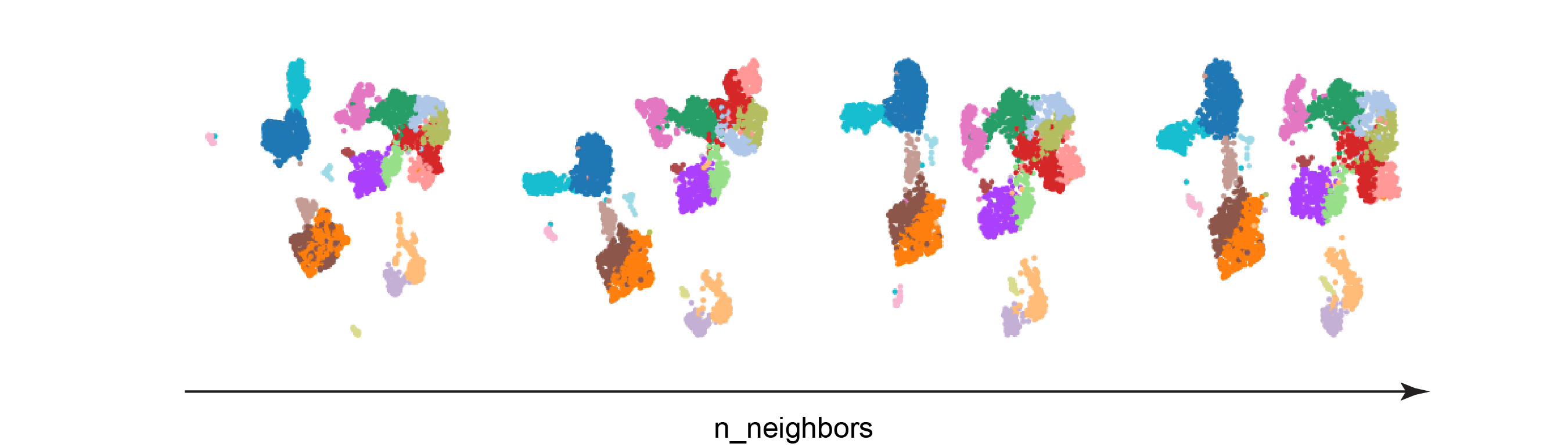
The resulting UMAPs look quite similar, but they do have some clear distinctions. As n_neighbors increases, the clusters are encroaching upon each other. Interestingly, the blue cluster on the left side of the UMAPs appears to be completely separated from the rest of the clusters only in the left-most UMAP. Larger values of min_dist may cause rare cell populations to get mixed into other cell types, since their spatial assignment would be more influenced by the global data landscape.

Test 2: min_dist and spread

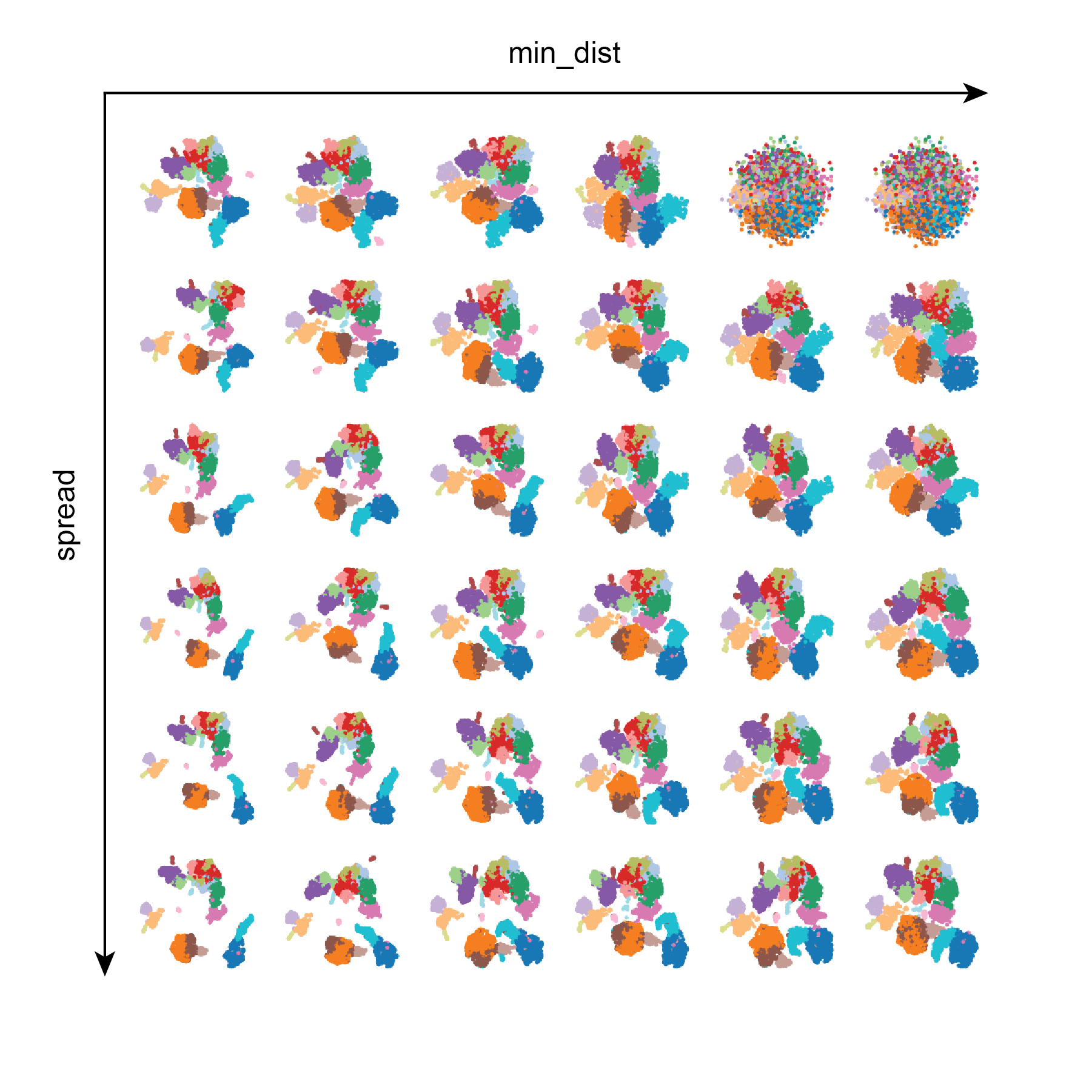
Here we can see that in general min_dist and spread influence the distance between points in the UMAP embedding, and that large values of min_dist results in the UMAP looking like a messy blob. In contrast, larger values of spread yield tighter clustering. In this dataset lower values of min_dist seem desirable in order to separate different cell populations in low dimensional space.

Test 3: gamma and alpha

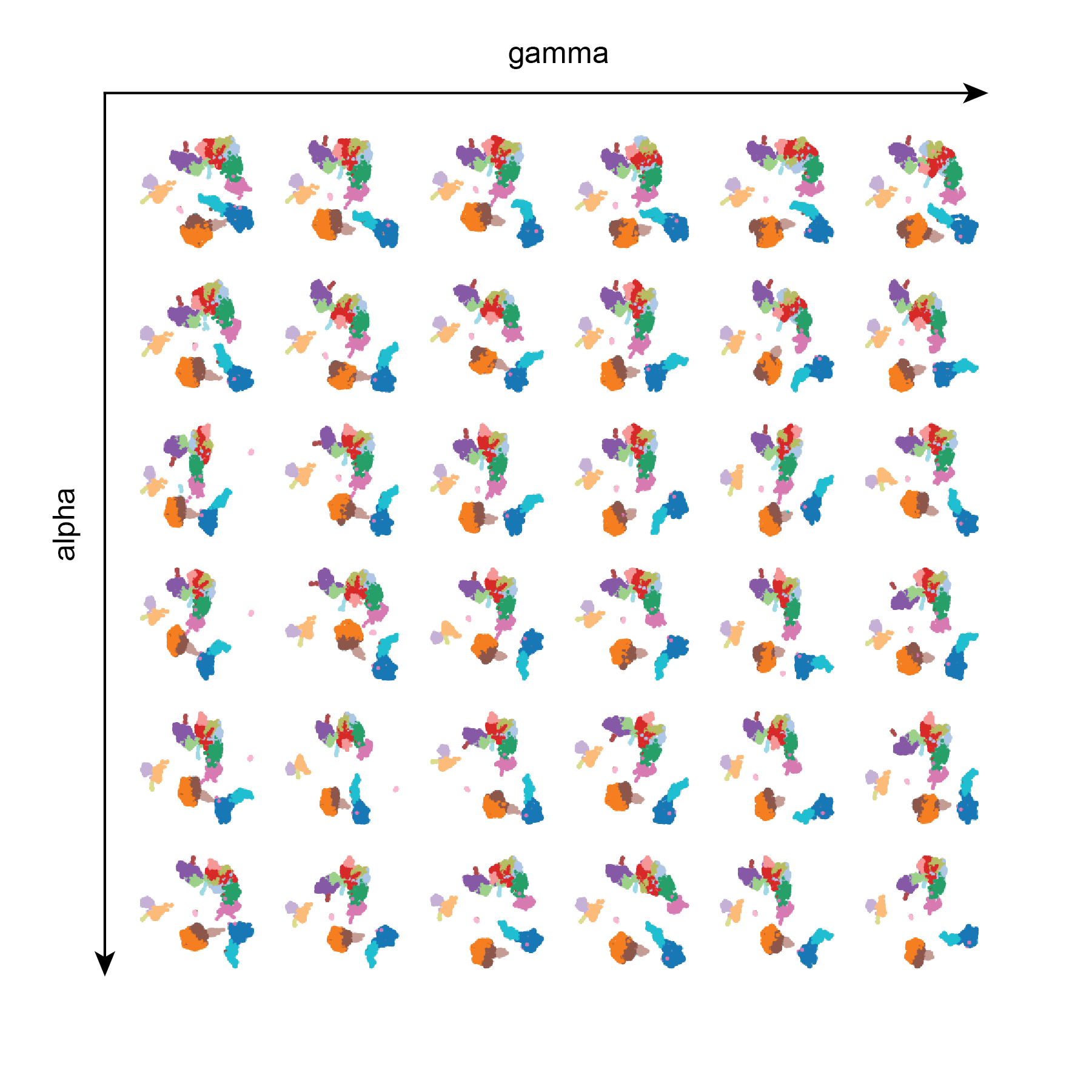
alpha and gamma do not appear to have very much influence on the resulting UMAPs. Perhaps more extreme values need to be tested, or perhaps a larger dataset should be used.

Test 4: maxiter and negative_sample_rate

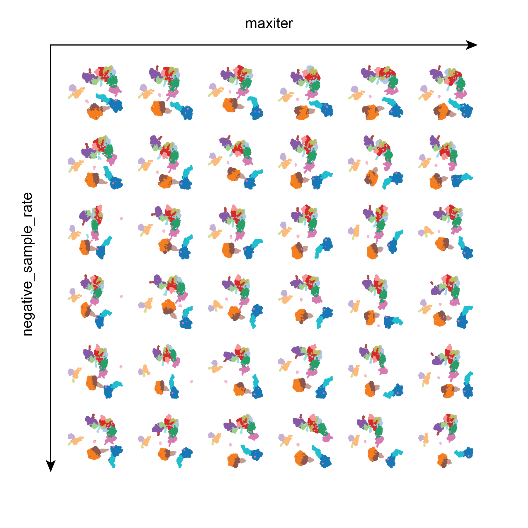
Similar to Test 3, maxiter and negative_sample_rate do not appear to have very much influence on the resulting UMAPs. This is helpful to know that it does not take a large amount of training iterations to achieve a decent UMAP.

Conclusion

In most cases it seems like it is okay to carry on using the default UMAP hyperparameters. If anything should be changed to best suit a certain dataset, the parameters that are going to have the most influence on the output are n_neighbors, and spread/min_dist. Perhaps it would be more informative to test a wider range of values, and to use different sized datasets (future blog post maybe). Take note that different software packages may have slightly different default parameters for UMAP.