Module perturbation on a branching trajectory

Compiled: 2026-05-21

Source: vignettes/simulation_tutorial.Rmd

Introduction

compact (co-expression module perturbation analysis for cellular transcriptomes) is an R package for in-silico gene perturbation analysis in single-cell RNA-seq data. compact builds on hdWGCNA, our previous package for weighted gene co-expression network analysis in single-cell data. If you are unfamiliar with co-expression modules or need to run hdWGCNA yourself, we recommend starting with the hdWGCNA tutorial.

Setup and data loading

For this tutorial, we use a splatter simulated scRNA-seq dataset of ~4,800 cells and ~6,000 genes. We simulated 3 distinct branches with 4 cell populations each to recapitulate a branching developmental trajectory. First, we will load the required libraries (Seurat, hdWGCNA, compact, etc) and the simulated dataset.

Prerequisite: The dataset used here already has co-expression modules computed with hdWGCNA. If you need to run hdWGCNA on your own data first, start with the hdWGCNA tutorial. Optionally you can expand the section below to see how the dataset was generated and preprocessed.

Dataset generation: simulation and preprocessing steps (click to expand)

The dataset was generated synthetically using splatter to simulate a branching single-cell trajectory, then processed through Seurat, Monocle3, and hdWGCNA. These steps are provided here for full reproducibility; they do not need to be re-run if you are loading the pre-processed object.

Create a simulated scRNA-seq dataset with a branching trajectory

library(Seurat)
library(tidyverse)
library(cowplot)
library(patchwork)
library(hdWGCNA)
library(compact)

theme_set(theme_cowplot())
set.seed(12345)

library(splatter)
library(scater)

params <- newSplatParams()
params <- setParam(params, "nGenes", 6000)
params <- setParam(params, "batchCells", 4800)
params <- setParam(params, "lib.loc", 8)

# three-branch path: shared root bifurcates twice into 12 ordered groups
path <- c(0, 1, 2, 2, 3, 5, 6, 7, 3, 9, 10, 11)

sim_path <- splatSimulatePaths(
    params,
    group.prob = rep(1 / length(path), length(path)),
    de.prob    = 0.75,
    de.facLoc  = 0.2,
    path.from  = path,
    verbose    = FALSE
)

# remove genes with no zero counts (fully non-sparse genes confound ZINB modeling)
X <- counts(sim_path)
exclude_genes <- names(which(rowMins(X) > 0))
X <- X[setdiff(rownames(X), exclude_genes), ]

seurat_obj <- CreateSeuratObject(
    counts    = X,
    meta.data = as.data.frame(colData(sim_path))
)

Process the data with Seurat

seurat_obj <- NormalizeData(seurat_obj)
seurat_obj <- FindVariableFeatures(seurat_obj)
seurat_obj <- ScaleData(seurat_obj)
seurat_obj <- RunPCA(seurat_obj)

Calculate the pseudotime trajectory with monocle3

library(monocle3)
library(SeuratWrappers)

# convert to CDS and reuse PCA coordinates as the 2D embedding for graph learning
cds <- as.cell_data_set(seurat_obj)
cds@int_colData@listData$reducedDims@listData$UMAP <-
    cds@int_colData@listData$reducedDims$PCA[, 1:2]

cds <- cluster_cells(cds, reduction_method = 'UMAP')
cds <- learn_graph(cds)

# root principal node identified by visual inspection of the learned graph
cds <- order_cells(cds, root_pr_nodes = 'Y_49')
seurat_obj$pseudotime <- pseudotime(cds)

# assign branch labels
branch0 <- c('Path1', 'Path2', 'Path3', 'Path4')
branch1 <- c('Path5', 'Path6', 'Path7', 'Path8')
branch2 <- c('Path9', 'Path10', 'Path11', 'Path12')

seurat_obj$branch <- case_when(
    seurat_obj$Group %in% branch0 ~ 'Branch 1',
    seurat_obj$Group %in% branch1 ~ 'Branch 2',
    seurat_obj$Group %in% branch2 ~ 'Branch 3'
)

# branch-specific pseudotime (NA for cells outside each branch)
b1_path <- c('Path1', 'Path2', 'Path3', 'Path4', 'Path5', 'Path6', 'Path7', 'Path8')
b2_path <- c('Path1', 'Path2', 'Path3', 'Path4', 'Path9', 'Path10', 'Path11', 'Path12')
seurat_obj$b1_pseudotime <- ifelse(seurat_obj$Group %in% b1_path, seurat_obj$pseudotime, NA)
seurat_obj$b2_pseudotime <- ifelse(seurat_obj$Group %in% b2_path, seurat_obj$pseudotime, NA)

# rename splatter path labels to human-readable branch-position labels
seurat_obj@meta.data <- seurat_obj@meta.data %>%
    mutate(Group = recode(Group,
        "Path1"  = "B1-1",  "Path2"  = "B1-2",  "Path4"  = "B1-3",  "Path3"  = "B1-4",
        "Path5"  = "B2-1",  "Path6"  = "B2-2",  "Path7"  = "B2-3",  "Path8"  = "B2-4",
        "Path9"  = "B3-1",  "Path10" = "B3-2",  "Path11" = "B3-3",  "Path12" = "B3-4"
    ))

Co-expression network analysis with hdWGCNA

seurat_obj <- SetupForWGCNA(
    seurat_obj,
    gene_select = "fraction",
    fraction    = 0.05,
    wgcna_name  = "simulation",
    group.by    = 'Group'
)

seurat_obj <- MetacellsByGroups(
    seurat_obj       = seurat_obj,
    group.by         = c("Group"),
    reduction        = 'pca',
    k                = 25,
    max_shared       = 10,
    ident.group      = 'Group',
    target_metacells = 50
)
seurat_obj <- NormalizeMetacells(seurat_obj)
seurat_obj <- SetDatExpr(seurat_obj)
seurat_obj <- TestSoftPowers(seurat_obj)

seurat_obj <- ConstructNetwork(
    seurat_obj,
    tom_name      = 'sim',
    overwrite_tom = TRUE
)

seurat_obj <- ModuleEigengenes(seurat_obj, group.by = 'branch')
seurat_obj <- ModuleConnectivity(seurat_obj)

saveRDS(seurat_obj, file = file.path(data_dir, 'simulation_branch.rds'))

Loading the dataset and required libraries

Start by loading the required libraries:

library(Seurat)
library(tidyverse)
library(cowplot)
library(patchwork)
library(RColorBrewer)
library(hdWGCNA)
library(compact)

theme_set(theme_cowplot())
set.seed(12345)

The dataset for this tutorial must be downloaded separately from Zenodo.

• simulation_branch.rds (Seurat object, ~50 MB) — Download from Zenodo
• sim_TOM.rda (co-expression network TOM, ~5 MB) — Download from Zenodo

After downloading, set data_dir to the folder containing both files and load the data:

# set this to the directory where you downloaded the data files
data_dir <- '/path/to/your/data/'

seurat_obj <- readRDS(file.path(data_dir, 'simulation_branch.rds'))

# register the TOM file path inside the Seurat object
net <- GetNetworkData(seurat_obj)
net$TOMFiles <- file.path(data_dir, 'sim_TOM.rda')
seurat_obj <- SetNetworkData(seurat_obj, net)

Plot the clusters

We familiarize ourselves with the dataset by plotting the different groups as a PCA dimensional reduction plot.

cp <- c(
    rev(brewer.pal(5, "Oranges")[2:5]),  # Branch 1: B1-1, B1-2, B1-3, B1-4
    brewer.pal(5, "Greens")[2:5],        # Branch 2: B2-1, B2-2, B2-3, B2-4
    brewer.pal(5, "Purples")[2:5]        # Branch 3: B3-1, B3-2, B3-3, B3-4
)
names(cp) <- c(
    'B1-1', 'B1-2', 'B1-3', 'B1-4',
    'B2-1', 'B2-2', 'B2-3', 'B2-4',
    'B3-1', 'B3-2', 'B3-3', 'B3-4'
)

DimPlot(
    seurat_obj,
    reduction = 'pca',
    group.by = 'Group',
    cols = cp,
    label = FALSE,
    pt.size = 1
) + coord_equal() 

Plot module eigengenes

We next inspect the expression level of each gene co-expression module identified by hdWGCNA.

plot_list <- ModuleFeaturePlot(
    seurat_obj,
    reduction = 'pca',
    features = 'MEs',
    order = TRUE
)
#> [1] "yellow"
#> [1] "brown"
#> [1] "blue"
#> [1] "red"
#> [1] "green"
#> [1] "turquoise"

wrap_plots(plot_list, ncol = 3)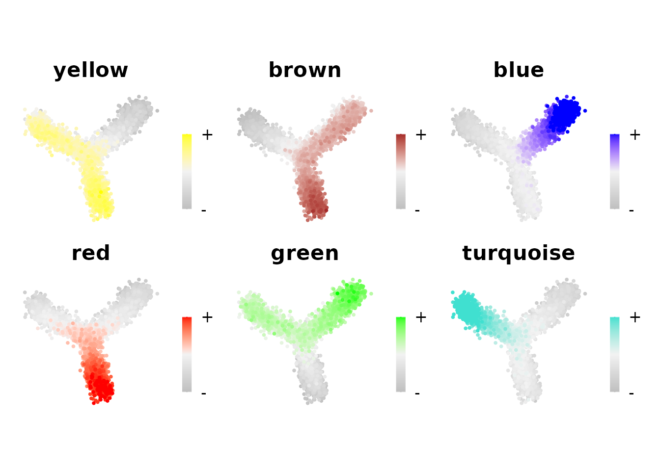

hdWGCNA identified six modules in this dataset. Three are specifically expressed in one branch (blue, red, and turquoise), while the other three are specifically inactive in one branch (yellow, brown, and green). In this tutorial, we focus on perturbing the turquoise module with compact.

---

Build the cell-cell neighborhood graph

Before running ModulePerturbation, we must construct a nearest-neighbor graph. This graph defines the local neighborhoods over which compact computes cell-cell transition probabilities. Essentially, transition probabilities are only computed between neighboring cells in the graph.

Run FindNeighbors to build the SNN (shared nearest neighbor) graph:

seurat_obj <- FindNeighbors(
    seurat_obj,
    reduction = 'pca',
    assay = 'RNA',
    k.param = 20,
    annoy.metric = 'cosine'
)

Parameters:

• k.param = 20: Each cell connects to its 20 nearest neighbors in PCA space. For datasets with 1,000s of cells, values between 15 and 50 typically work well; for smaller datasets, lower values are appropriate.
• annoy.metric = 'cosine': Use cosine distance (standard for high-dimensional gene expression data). Alternative: 'euclidean'.
• reduction = 'pca': Compute neighbors in PCA space rather than the full gene expression matrix (more efficient and robust).

The SNN graph is stored in the Seurat object at seurat_obj@graphs[['RNA_snn']]. This is the graph ModulePerturbation will use to compute transition probabilities in the next section.

Note: The graph is only computed once, even if you perform multiple perturbations. You can run ModulePerturbation sequentially for different modules or different perturbation directions without re-running FindNeighbors.

Checking graph connectivity

A critical requirement is that the SNN graph should be fully connected every cell should be reachable from every other cell through the graph edges. If the graph has isolated components, transition probability mass is trapped within those regions during ModulePerturbation, producing artefactual attractor states or flat pseudotime values in disconnected areas.

The choice of k.param has the largest effect on connectivity. Too few neighbors leaves sparse or peripheral cells with no shared-neighbor edges after SNN pruning, splitting the graph into isolated pieces. Too many neighbors blurs local neighborhood structure. We recommend sweeping a few candidate values and checking connectivity with FindConnectedComponents before committing to a final graph.

compact provides FindConnectedComponents to detect this condition. It labels each cell by its connected component and warns you if more than one is found. Below we run FindNeighbors with four representative k.param values and save the component labels from each run under a unique column name, allowing us to compare all four results side-by-side:

param_sets <- list(
    list(k = 2,  label = 'k2'),
    list(k = 10, label = 'k10'),
    list(k = 20, label = 'k20'),
    list(k = 50, label = 'k50')
)

for (ps in param_sets) {
    seurat_obj <- FindNeighbors(
        seurat_obj,
        reduction    = 'pca',
        assay        = 'RNA',
        k.param      = ps$k,
        annoy.metric = 'cosine',
        verbose      = FALSE
    )
    seurat_obj <- FindConnectedComponents(
        seurat_obj,
        graph          = 'RNA_snn',
        meta_data_name = paste0('cc_', ps$label),
        verbose        = FALSE
    )
}

We can now visualize the results side-by-side.

plot_list <- lapply(param_sets, function(ps) {
    col_name <- paste0('cc_', ps$label)
    n_comp   <- nlevels(seurat_obj@meta.data[[col_name]])
    status   <- if (n_comp == 1) '1 component' else paste0(n_comp, ' components')

    DimPlot(
        seurat_obj,
        reduction = 'pca',
        group.by  = col_name,
        pt.size   = 0.5
    ) +
        coord_equal() +
        NoLegend() +
        ggtitle(paste0('k=', ps$k, '  (', status, ')'))
})

wrap_plots(plot_list, ncol = 2)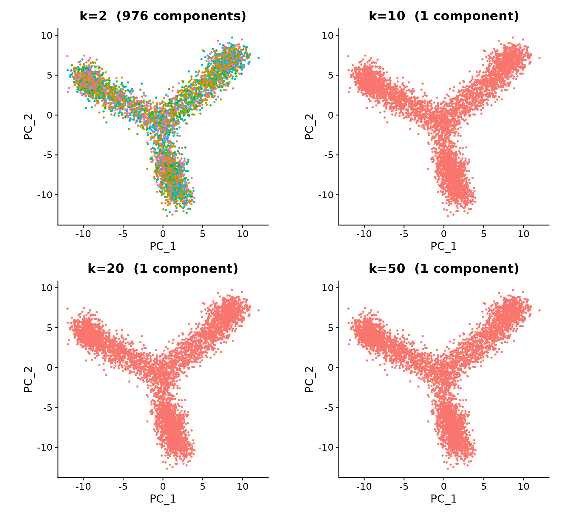

In this example, k.param = 2 was the only tested value that yielded more than one component, although this is an unrealistically low value to use in a practical setting.

Note: In the case where multiple components are detected using a higher k.param value, we advise that the user consider subsetting their object to only perform the downstream analysis on a single connected component of the graph.

For this dataset, we proceed with k.param = 20.

seurat_obj <- FindNeighbors(
    seurat_obj,
    reduction    = 'pca',
    assay        = 'RNA',
    k.param      = 20,
    annoy.metric = 'cosine'
)
seurat_obj <- FindConnectedComponents(
    seurat_obj,
    graph   = 'RNA_snn'
)

---

Running ModulePerturbation

Here we run ModulePerturbation, the core function of compact, to perform an in-silico down-regulation and up-regulation of the turquoise module. This function performs three sequential steps internally:

1. ApplyPerturbation: Directly modifies the gene expression counts of the top hub genes in the target co-expression module in the direction specified by perturb_dir.
2. ApplyPropagation: Propagates that initial perturbation signal on the hub genes through the rest of the co-expression network, updating the expression of all genes connected to the hub genes.
3. PerturbationTransitions: Computes cell-cell transition probabilities on a cell-cell nearest neighbors graph using the perturbed expression matrix, yielding a transition probability matrix analogous to those from RNA velocity.

The results are stored back into the Seurat object as a new assay (the perturbed expression) and a new graph (the transition probability matrix).

Down-regulation (knock-down)

compact defaults to ZINB mode (perturb_mode = "zinb"), which models each hub gene’s baseline expression with a Zero-Inflated Negative Binomial distribution and adds (knock-in) or subtracts (knock-down) a sample from that distribution. For knock-down, set perturb_dir = -1; for knock-in, set perturb_dir = 1; for knock-out (force expression to zero), set perturb_dir = 0.

cur_mod <- 'turquoise'

seurat_obj <- ModulePerturbation(
    seurat_obj,
    mod = cur_mod,
    perturb_dir = -1,
    perturbation_name = 'turquoise_down',
    group.by = 'Group',
    graph = 'RNA_snn',
    n_hubs = 10,
    delta_scale = 1.0,
    row_normalize = FALSE,
    use_velocyto = FALSE,
    n_workers = 1
)
#> [1] "Applying primary in-silico perturbation to hub genes..."
#>   |                                                          |                                                  |   0%  |                                                          |=====                                             |  10%  |                                                          |==========                                        |  20%  |                                                          |===============                                   |  30%  |                                                          |====================                              |  40%  |                                                          |=========================                         |  50%  |                                                          |==============================                    |  60%  |                                                          |===================================               |  70%  |                                                          |========================================          |  80%  |                                                          |=============================================     |  90%  |                                                          |==================================================| 100%
#> [1] "Applying log-space signal propagation throughout co-expression network..."
#> [1] "Computing cell-cell transition probabilities based on the perturbation..."

Up-regulation (knock-in)

We set perturb_dir = 1 to simulate over-expression of the module, holding all other parameters the same as the down-regulation case.

seurat_obj <- ModulePerturbation(
    seurat_obj,
    mod = cur_mod,
    perturb_dir = 1,
    perturbation_name = 'turquoise_up',
    group.by = 'Group',
    graph = 'RNA_snn',
    n_hubs = 10,
    delta_scale = 1.0,
    row_normalize = FALSE,
    use_velocyto = FALSE,
    n_workers = 1, 
    n_iters = 1
)
#> [1] "Applying primary in-silico perturbation to hub genes..."
#>   |                                                          |                                                  |   0%  |                                                          |=====                                             |  10%  |                                                          |==========                                        |  20%  |                                                          |===============                                   |  30%  |                                                          |====================                              |  40%  |                                                          |=========================                         |  50%  |                                                          |==============================                    |  60%  |                                                          |===================================               |  70%  |                                                          |========================================          |  80%  |                                                          |=============================================     |  90%  |                                                          |==================================================| 100%
#> [1] "Applying log-space signal propagation throughout co-expression network..."
#> [1] "Computing cell-cell transition probabilities based on the perturbation..."

Looping over all modules

To systematically perform perturbations over all modules, we can simply run a for loop across all the modules.

Running perturbations for all modules (click to expand)

To loop over all non-grey modules:

modules <- GetModules(seurat_obj)
mods <- unique(modules$module)
mods <- mods[mods != 'grey']

for (cur_mod in mods) {
    seurat_obj <- ModulePerturbation(
        seurat_obj,
        mod = cur_mod,
        perturb_dir = -1,
        perturbation_name = paste0(cur_mod, '_down'),
        group.by = 'Group',
        graph = 'RNA_snn',
        n_hubs = 10,
        delta_scale = 1.0,
        row_normalize = FALSE,
        use_velocyto = FALSE,
        n_workers = 1
    )
    seurat_obj <- ModulePerturbation(
        seurat_obj,
        mod = cur_mod,
        perturb_dir = 1,
        perturbation_name = paste0(cur_mod, '_up'),
        group.by = 'Group',
        graph = 'RNA_snn',
        n_hubs = 10,
        delta_scale = 1.0,
        row_normalize = FALSE,
        use_velocyto = FALSE,
        n_workers = 1
    )
}

Key parameters

• perturb_dir: -1 for knock-down, +1 for knock-in, 0 for knock-out.
• n_hubs = 10: The top 10 hub genes (by kME, module membership score) receive the primary perturbation; the signal diffuses to the rest of the network through ApplyPropagation.
• delta_scale = 1.0: Scaling factor for network propagation. The effective propagation magnitude depends on the density of the TOM (sum of edge weights per gene). When row_normalize = TRUE (see below), each propagation step is guaranteed to dampen the signal regardless of TOM density, so delta_scale = 1.0 is a safe default. Without row normalization, a smaller value (e.g. 0.01–0.05) may be needed to avoid saturation on dense networks. See ?ApplyPropagation for details.
• row_normalize = TRUE: Normalizes each row of the TOM to sum to 1 before propagation. This is recommended when working with dense networks (e.g. those built from simulated data or datasets with many co-expressed genes), where large row sums would otherwise cause signal amplification and floor-clipping across iterations.
• n_workers = 1: Number of parallel workers for fitting the ZINB model across hub genes. Set to a higher value (e.g., n_workers = 4) to speed up the computation on Unix/macOS. Note: n_workers > 1 uses fork-based parallelism (mclapply) and is not supported on Windows; on Windows, leave this at 1.

Note: The KNN graph is built once and reused. You can run ModulePerturbation for multiple modules or directions without re-running FindNeighbors.

After running both perturbations, the Seurat object contains two new assays (turquoise_down, turquoise_up) and two new transition probability graphs (turquoise_down_tp, turquoise_up_tp).

use_velocyto: This flag controls which implementation computes the cosine correlations inside PerturbationTransitions. The default (use_velocyto = FALSE) uses compact’s built-in SparseColDeltaCor, which operates on sparse matrices and only evaluates correlations for graph-connected cell pairs — making it memory-efficient and fast for large datasets. Setting use_velocyto = TRUE instead calls colDeltaCor from the velocyto.R package (which must be installed separately); this implementation requires expression matrices in dense format before computing correlations, so it is markedly slower and more memory-intensive but is provided for users who need to reproduce results from older compact analyses originally built on the velocyto implementation. The two implementations produce similar results but not numerically identical, since velocyto.R is calculating cell-cell transitions for every pair of cells in the dataset, while compact focuses only on cell-cell transitions for pairs of cells connected in the user-specified KNN or SNN graph.

Multiplicative mode

An alternative to the default ZINB model is perturb_mode = "multiplicative", which scales each cell’s observed counts directly by a user-specified fold change, bypassing distribution fitting entirely. In this mode perturb_dir is interpreted as a positive fold-change multiplier rather than a directional sign:

• Values between 0 and 1 reduce expression (e.g., 0.5 halves counts — knock-down equivalent)
• Values greater than 1 amplify expression (e.g., 2.0 doubles counts — knock-in equivalent)
• perturb_dir = 0 produces a knock-out in either mode

Code example for multiplicative mode (click to expand)

# multiplicative knock-down: reduce hub gene expression to 50%
seurat_obj <- ModulePerturbation(
    seurat_obj,
    mod               = cur_mod,
    perturb_dir       = 0.5,
    perturb_mode      = 'multiplicative',
    perturbation_name = 'turquoise_down_mult',
    group.by          = 'Group',
    graph             = 'RNA_snn',
    n_hubs            = 10,
    delta_scale       = 1.0,
    row_normalize     = TRUE,
    use_velocyto      = FALSE
)

# multiplicative knock-in: double hub gene expression
seurat_obj <- ModulePerturbation(
    seurat_obj,
    mod               = cur_mod,
    perturb_dir       = 2.0,
    perturb_mode      = 'multiplicative',
    perturbation_name = 'turquoise_up_mult',
    group.by          = 'Group',
    graph             = 'RNA_snn',
    n_hubs            = 10,
    delta_scale       = 1.0,
    row_normalize     = TRUE,
    use_velocyto      = FALSE
)

Multiplicative mode differs from ZINB mode in two important ways.

Speed. No per-gene distribution fitting is performed, so group.by and n_workers are both ignored and the computation is substantially faster — particularly useful when sweeping over many modules or working with large datasets.

Cell-specificity. Because the delta is proportional to each cell’s observed counts, cells with zero baseline expression are not affected. In ZINB mode, non-expressing cells can receive positive counts during knock-in because the sampled delta is drawn from a group-level distribution independent of that cell’s actual value. Multiplicative mode therefore better preserves the mathematical symmetry between knock-downs and knock-ins.

---

Inspecting expression changes

Before examining cell-state transitions, it is good practice to verify that the perturbation changed gene expression in the expected direction. This section shows two complementary views.

Violin plots of individual genes

We compare a top hub gene and a secondary module gene across the three conditions (observed, knock-down, knock-in), faceted by branch. Each column is a gene; each row is a branch. Significance brackets from a Wilcoxon test show whether knock-down and knock-in differ from the observed baseline within each branch.

library(ggpubr)

# get the top hub gene and a secondary gene
hub_genes     <- GetHubGenes(seurat_obj, n_hubs = 10)
module_genes  <- subset(GetModules(seurat_obj), module == cur_mod)$gene_name
hub_gene      <- subset(hub_genes, module == cur_mod)$gene_name[1]
secondary_gene <- module_genes[1]
genes_plot    <- c(hub_gene, secondary_gene)

# pull normalized expression from each assay and combine into a long data frame
get_expr_df <- function(assay_name, condition_label) {
    mat <- GetAssayData(seurat_obj, assay = assay_name, layer = 'data')
    df  <- as.data.frame(t(as.matrix(mat[genes_plot, , drop = FALSE])))
    df$condition <- condition_label
    df$branch    <- seurat_obj$branch
    df
}

plot_df <- bind_rows(
    get_expr_df('RNA',            'Observed'),
    get_expr_df('turquoise_down', 'Knock-down'),
    get_expr_df('turquoise_up',   'Knock-in')
) %>%
    pivot_longer(
        cols      = all_of(genes_plot),
        names_to  = 'gene',
        values_to = 'expression'
    ) %>%
    mutate(
        condition = factor(condition, levels = c('Observed', 'Knock-down', 'Knock-in')),
        gene      = factor(gene, levels = genes_plot)
    )

# significance brackets comparing each perturbation to observed
comparisons <- list(
    c('Observed', 'Knock-down'),
    c('Observed', 'Knock-in')
)

cond_colors <- c(
    'Observed'   = 'grey50',
    'Knock-down' = 'steelblue3',
    'Knock-in'   = 'firebrick3'
)

ggplot(plot_df, aes(x = condition, y = expression, color = condition)) +
    ggrastr::rasterise(ggbeeswarm::geom_quasirandom(
        method = 'pseudorandom',
        size   = 0.2,
        alpha  = 0.5
    ), dpi = 300) +
    geom_boxplot(
        outlier.shape = NA,
        alpha  = 0.3,
        color  = 'black',
        width  = 0.5
    ) +
    stat_compare_means(
        comparisons = comparisons,
        method      = 'wilcox.test',
        label       = 'p.signif',
        size        = 3,
        tip.length  = 0.01
    ) +
    scale_color_manual(values = cond_colors) +
    facet_grid(branch ~ gene, scales = 'free_y') +
    theme(
        axis.text.x        = element_text(angle = 45, hjust = 1),
        panel.border       = element_rect(linewidth = 1, color = 'black', fill = NA),
        panel.grid.major.y = element_line(linewidth = 0.25, color = 'lightgrey'),
        strip.text         = element_text(size = 9)
    ) +
    NoLegend() +
    xlab('') + ylab('Normalized expression')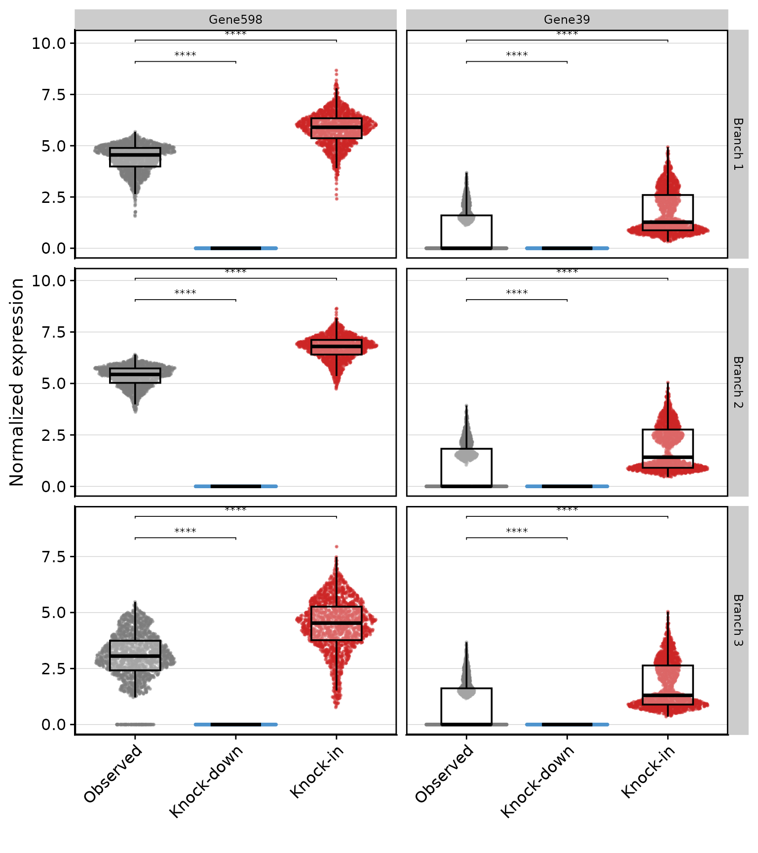

Hub genes (left column) should show the largest effect sizes — they are the primary targets of the perturbation. Secondary module genes (right column) show smaller but consistent changes, reflecting signal propagated through the co-expression network. The turquoise module is most highly expressed on Branch 1, so that row is expected to show the strongest and most significant differences.

Perturbed vs. observed log2FC (click to expand)

PerturbationLog2FC computes the log2 fold change for all genes in a module, comparing the perturbed assay to the baseline. Here we simply show how to access this information using the compact function PerturbationLog2FC.

library(ggrepel)

lfc_down <- PerturbationLog2FC(
    seurat_obj,
    perturbation_name = 'turquoise_down',
    module = cur_mod,
    n_hubs = 10
)

knitr::kable(
    head(lfc_down, 10),
    digits    = 4
)

gene_name	mean_delta	avg_exp	log2fc	module	kME	hub
Gene598	-26.9231	4.2385	-2.3891	turquoise	0.7392	hub
Gene2479	-8.2340	3.2091	-2.0735	turquoise	0.6734	hub
Gene90	-10.6802	3.5795	-2.1952	turquoise	0.6647	hub
Gene4743	-2.1229	1.7936	-1.4821	turquoise	0.6070	hub
Gene2261	-2.9592	2.3361	-1.7382	turquoise	0.6012	hub
Gene4541	-9.2560	3.5568	-2.1880	turquoise	0.5957	hub
Gene320	-12.5417	3.8910	-2.2901	turquoise	0.5801	hub
Gene3914	-4.9246	2.8562	-1.9472	turquoise	0.5721	hub
Gene4351	-19.6294	4.3462	-2.4185	turquoise	0.5672	hub
Gene4010	-18.2354	4.2127	-2.3820	turquoise	0.5648	hub

Note: In the case of this simulated dataset, the log2FCs of non-hub genes are very low in the current parameter regime. This is partially due to the abnormally dense nature of the co-expression matrix itself in a simulated dataset. We show more biologically realistic log2FC values in the tutorial on non-simulated data.

---

Transition vector fields

PlotTransitionVectors projects the cell-cell transition probabilities onto the two-dimensional embedding as a vector field. While this visualization resembles an RNA velocity plot, the vector field in this context summarizes the local directional change of a cell under a specific in-silico perturbation, while RNA velocity aims to show a cell’s “natural” trajectory based on ratios of spliced to unspliced transcripts. Each arrow on the grid represents the weighted average direction of transitions in that region of the embedding.

The points are colored by the turquoise module eigengene, so you can see where turquoise module is expressed at baseline relative to where the arrows are pointing.

# extract the module color for turquoise
modules <- GetModules(seurat_obj)
mod_colors <- dplyr::select(modules, module, color) %>% dplyr::distinct()
mod_cp <- setNames(mod_colors$color, mod_colors$module)
cur_mod_color <- mod_cp[cur_mod]

# knock-down vector field
p_down <- PlotTransitionVectors(
    seurat_obj,
    perturbation_name = 'turquoise_down',
    reduction = 'pca',
    color.by = cur_mod,
    grid_resolution = 25,
    arrow_scale = 2,
    point_alpha = 0.9,
    point_size = 3,
    arrow_size = 0.4,
    max_pct = 0.5,
    arrow_alpha = TRUE
) +
    NoLegend() +
    scale_color_gradient2(high = cur_mod_color, low = 'whitesmoke', mid = 'whitesmoke') +
    ggtitle('turquoise, knock-down') +
    coord_equal()

# knock-in vector field
p_up <- PlotTransitionVectors(
    seurat_obj,
    perturbation_name = 'turquoise_up',
    reduction = 'pca',
    color.by = cur_mod,
    grid_resolution = 25,
    arrow_scale = 2,
    point_alpha = 0.9,
    point_size = 3,
    arrow_size = 0.4,
    max_pct = 0.5,
    arrow_alpha = TRUE
) +
    NoLegend() +
    scale_color_gradient2(high = cur_mod_color, low = 'whitesmoke', mid = 'whitesmoke') +
    ggtitle('turquoise, knock-in') +
    coord_equal()

p_down + p_up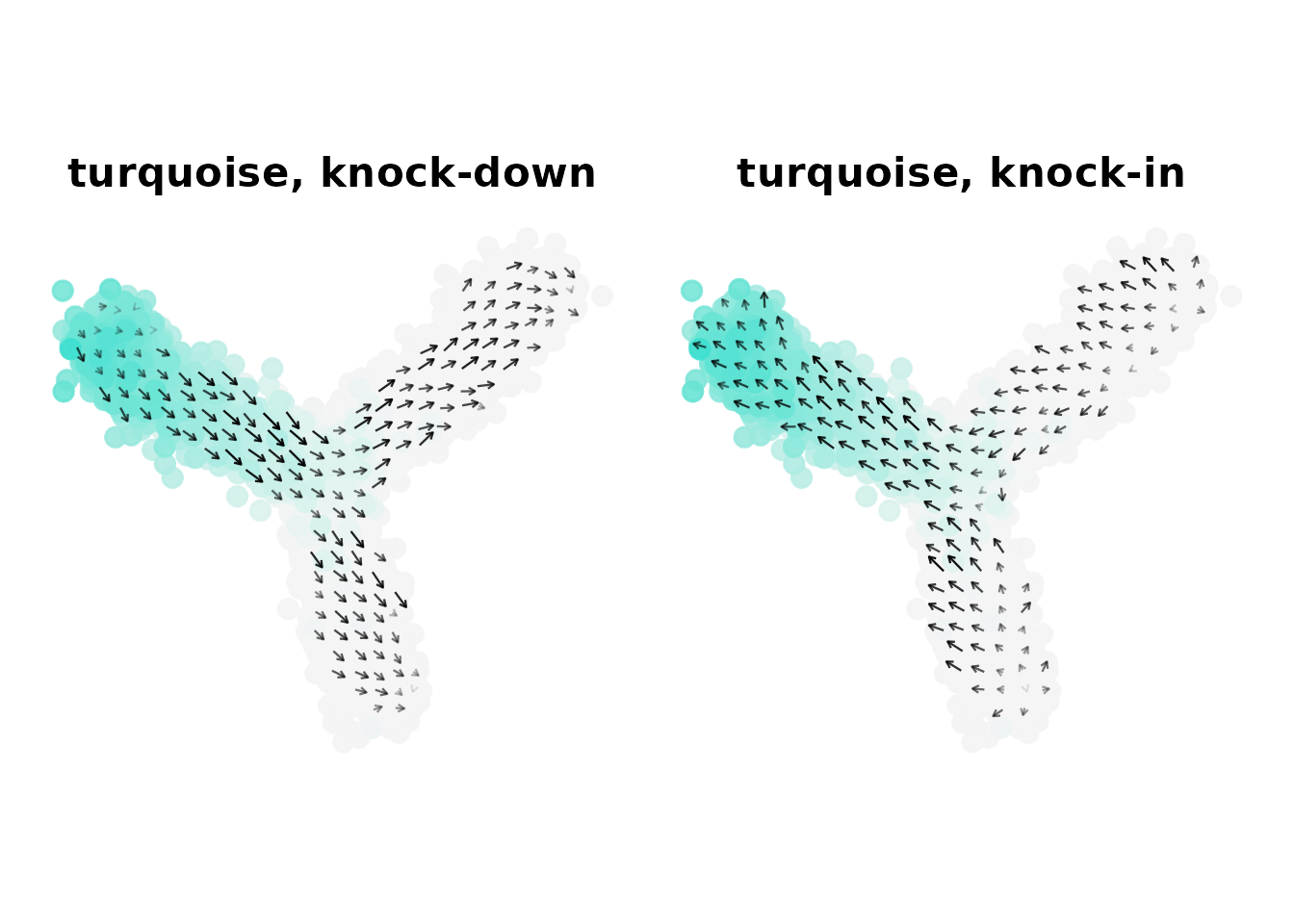

What to look for: The two vector fields should be roughly opposite. In the region where turquoise expression is highest (bright-colored cells), knock-down arrows should point away from that region, and knock-in arrows should point toward it. The perturbation shifts cell-state transitions in the direction consistent with the module’s role in defining the underlying trajectory.

Key parameters:

• grid_resolution = 25: Number of grid points along each axis. Higher values give finer spatial resolution but can be noisy with few cells per grid square.
• arrow_scale = 2: Scales the displayed arrow length for visual clarity; does not affect underlying transition probabilities.
• max_pct = 0.5: Trims the top 50% of arrow magnitudes before scaling, preventing a few extreme arrows from dominating the visualization.
• arrow_alpha = TRUE: Fades arrows with smaller magnitudes so that stronger transitions stand out visually.

Vector field coherence

Two-dimensional embeddings like UMAP invariably introduce global distortions in the underlying dataset, and therefore we must avoid over-interpretation of the results in a two-dimensional setting. VectorFieldCoherence quantifies how locally consistent the perturbation signal is across the embedding. For each cell, it computes the cosine similarity between that cell’s perturbation vector and those of its neighbors in the cell-cell neighborhod graph. Coherence ranges from −1 (perfectly anti-aligned with neighbors) to +1 (perfectly aligned), with values near 0 indicating random or mixed directions.

High coherence in a region means the perturbation consistently pushes cells in the same direction there. Low coherence may indicate cells with low module expression or cells in a transition zone between two cell states.

seurat_obj$coherence_down <- VectorFieldCoherence(
    seurat_obj,
    perturbation_name = 'turquoise_down',
    reduction = 'pca',
    graph = 'RNA_snn',
    weighted = TRUE
)

seurat_obj$coherence_up <- VectorFieldCoherence(
    seurat_obj,
    perturbation_name = 'turquoise_up',
    reduction = 'pca',
    graph = 'RNA_snn',
    weighted = TRUE
)

We can visualize coherence directly on the embedding, but here we plot the distributions of these values by group and branch:

plot_df <- as.data.frame(Reductions(seurat_obj, 'pca')@cell.embeddings[, 1:2])
plot_df$coherence <- seurat_obj$coherence_down
plot_df$Group <- seurat_obj$Group
plot_df$branch <- seurat_obj$branch

# rank groups by median coherence for display
group_order <- plot_df %>%
    group_by(Group) %>%
    summarise(med = median(coherence)) %>%
    arrange(med) %>%
    pull(Group)
plot_df$Group <- factor(plot_df$Group, levels = group_order)

p <- plot_df %>%
    ggplot(aes(x=coherence, y=Group, color=Group)) +
    ggrastr::rasterise(ggbeeswarm::geom_quasirandom(
        method = "pseudorandom",
        size=0.25
    ), dpi=300) +
    geom_boxplot(outlier.shape=NA, alpha=0.3, color='black') +
    scale_color_manual(values=cp) +
    theme(
            axis.line.x = element_blank(),
            axis.line.y = element_blank(),
            axis.ticks.x = element_line(linewidth=0.5),
            axis.ticks.y = element_line(linewidth=0.5),
            panel.border = element_rect(linewidth=1,color='black', fill=NA),
            strip.text = element_blank(),
            plot.title = element_text(hjust=0.5) 
    ) +
    NoLegend() + 
    xlab('Local coherence') + ylab("") + 
    ggtitle('turquoise knock-down') +
    xlim(c(-1,1))

p + facet_wrap(vars(branch), ncol=1, scales='free_y')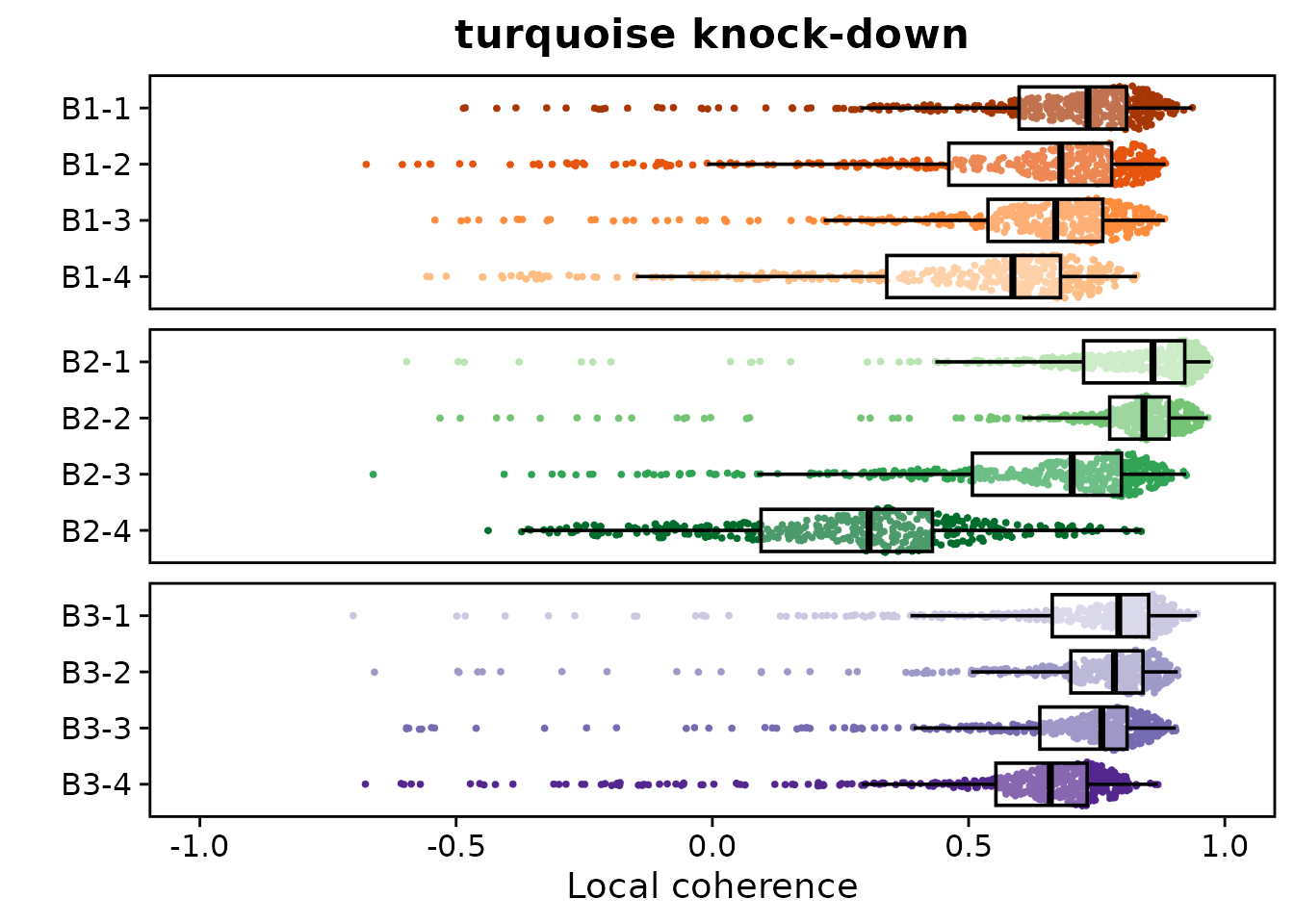

This analysis shows generally high local coherence of the perturbation vectors across all branches and individual groups, meaning that transcriptomically similar cells (ie, connected in the cell-cell neighborhood graph) overall respond similarly to the perturbation. Ultimately each cell and each cluster is unique, so there remains dynamic range of coherence values across groups.

---

Macrostate transitions

PlotTransitionVectors shows per-cell transition directions projected onto the UMAP — informative but inherently limited by embedding distortions. MacrostateTransitions provides a complementary embedding-independent view: it coarse-grains the full-dimensional transition probability matrix into a K × K group-level summary, answering the question “on average, when a cell in group A transitions, where does it go?” Here the “macrostates” are simply the previously defined cell clusters.

The result is a matrix Q where each entry Q[source, destination] is the mean transition probability from any cell in the source group to any cell in the destination group. The diagonal of Q is the stability index — the fraction of a group’s outgoing transitions that stay within the same group. A stability close to 1 signals an attractor-like state that resists the perturbation; low stability marks a transient source population whose cells are being redirected elsewhere.

Run MacrostateTransitions

# down-regulation
seurat_obj <- MacrostateTransitions(
    seurat_obj,
    perturbation_name = 'turquoise_down',
    graph             = 'RNA_snn',
    group.by          = 'Group'
)

seurat_obj <- MacrostateTransitions(
    seurat_obj,
    perturbation_name = 'turquoise_up',
    graph             = 'RNA_snn',
    group.by          = 'Group'
)

# arrange groups in trajectory order so the heatmap reads root → tip left-to-right
group_order <- c(
    'B1-1', 'B1-2', 'B1-3', 'B1-4',
    'B2-1', 'B2-2', 'B2-3', 'B2-4',
    'B3-1', 'B3-2', 'B3-3', 'B3-4'
)

PlotMacrostateTransitions(
    seurat_obj,
    perturbation_name = 'turquoise_down',
    group_order       = group_order,
    title             = 'Turquoise knock-down — macrostate transitions'
)

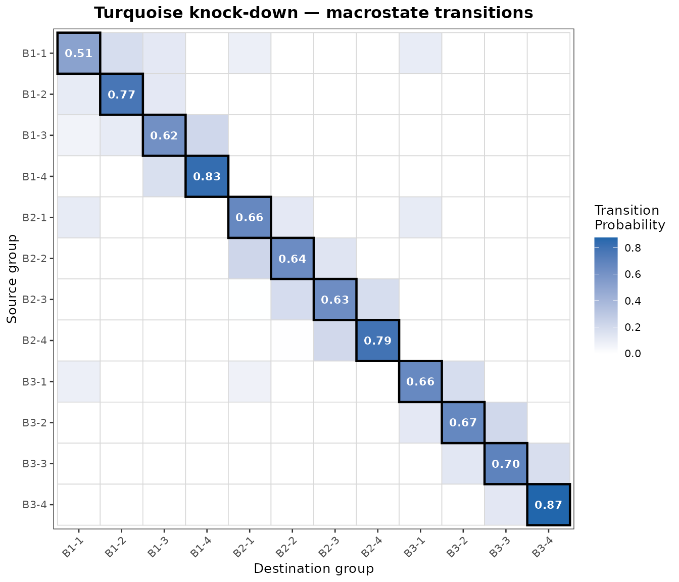
To interpret this plot, we can read the heatmap row by row. Each row corresponds to a “source” group; the tile intensities tell you where the cells are predicted to transition. For example, for the top row (group B1-1) aside from remaining within the same group, under this perturbation the cells are likely to transition to group B2-2, but to no other groups. This makes intuitive sense when we consider the PCA DimPlot from earlier, the only “neighboring” cluster to B1-1 is in fact B1-2.

In general, we observe strong diagonal tiles in the heatmap, showing self-transition probability. This is expected since cells within the same group have the densest connections within the cell-cell network. The strong off-diagonal tiles are more interesting in this case as they show the predicted shifts from one group to another under this perturbation.

---

Perturbation cell fate analysis

compact provides several functions that together aim to interrogate the downstream consequences of in-silico perturbations on cell fates. In particular, we treat the transition probability matrix as a Markov chain and extract different types of cell-fate information. We demonstrate each of these functions using the knock-down perturbation of the turquoise module.

• PredictAttractors identifies natural sink states from the stationary distribution
• PredictPerturbationTime computes an absorbing-chain hitting time (perturbation pseudotime)
• PredictFates calculates forward-diffusion fate probabilities toward a target population
• PredictCommitment computes the committor probability between two competing cell states.

In general, these functions provide cell-level outputs which we can then visualize using different approaches. compact provides a built-in visualization solution, PlotMarkovEmbedding, which you can consider as a specialized form of the Seurat FeaturePlot function with some additional functionality for this analysis in particular. For instance, source and sink populations can be explicitly marked with a single centroid diamond per group (labeled automatically with ggrepel), making their positions clear without cluttering the plot; and unconverged cells (those that hit max_iter in iterative solvers) are drawn in grey below the color scale rather than receiving a misleading color value.

Shared setup: defining sink cells

For several of the analyses below, we must specify sink cells, a set of cells that serve as absorbing states in the Markov chain. We define them simply as all cells in the earliest pseudotime group, B1-1, which sits at the shared root region of the trajectory:

perturb_name <- 'turquoise_down'

# define sink cells by group membership (root of the trajectory)
sink_cells <- colnames(seurat_obj)[seurat_obj$Group == 'B1-4']

Identifying attractor states

PredictAttractors computes the stationary distribution of the transition probability Markov chain, which represents the probability of finding the Markov random walk at each cell. Cells with high stationary probability act as attractors, or natural “sinks,” in the perturbation dynamics.

Setting return_seurat = FALSE returns a list with both the continuous stationary-distribution scores and the binary sink-cell membership. We then compute the ECDF transformation manually so we can store both the raw and the rank-normalized scores for comparison.

# return_seurat=FALSE gives us both the raw scores and the identified sink cells
attr_result <- PredictAttractors(
    seurat_obj,
    perturbation_name = perturb_name,
    graph             = 'RNA_snn',
    rank_transform    = FALSE,
    return_seurat     = FALSE
)

# store raw stationary-distribution scores
seurat_obj <- AddMetaData(seurat_obj,
    metadata = attr_result$attractor_score,
    col.name = 'attractor_score_raw'
)

# compute ECDF-normalized scores ([0,1] percentile ranks) and store separately
ecdf_scores <- ecdf(attr_result$attractor_score)(attr_result$attractor_score)
names(ecdf_scores) <- names(attr_result$attractor_score)
seurat_obj <- AddMetaData(seurat_obj,
    metadata = ecdf_scores,
    col.name = 'attractor_score'
)

# add binary attractor state (top 2% by default quantile_threshold = 0.98);
# factor levels are set so 'Other' is drawn first and 'Attractor' on top
seurat_obj$attractor_state <- factor(
    ifelse(colnames(seurat_obj) %in% attr_result$sink_cells, 'Attractor', 'Other'),
    levels = c('Other', 'Attractor')
)

Plotting the raw score alongside the ECDF-normalized version makes the benefit of the rank transformation visible: the raw stationary distribution has a heavy right tail concentrated on a handful of cells, while ECDF spreading stretches the color scale across the full manifold.

p_raw <- PlotMarkovEmbedding(
    seurat_obj,
    feature      = 'attractor_score_raw',
    reduction    = 'pca',
    sink_cells   = attr_result$sink_cells,
    sink_label   = 'Attractor cells',
    color_scale  = c('whitesmoke', 'darkorchid3'),
    pt_size      = 1.5,
    legend_title = 'Attractor score\n(raw)',
    title        = 'Raw stationary distribution'
) + coord_equal()

p_attractors <- PlotMarkovEmbedding(
    seurat_obj,
    feature      = 'attractor_score',
    reduction    = 'pca',
    sink_cells   = attr_result$sink_cells,
    sink_label   = 'Attractor cells',
    color_scale  = c('whitesmoke', 'darkorchid3'),
    pt_size      = 1.5,
    legend_title = 'Attractor score\n(ECDF)',
    title        = 'ECDF-normalized'
) + coord_equal()

wrap_plots(p_raw, p_attractors, ncol = 2)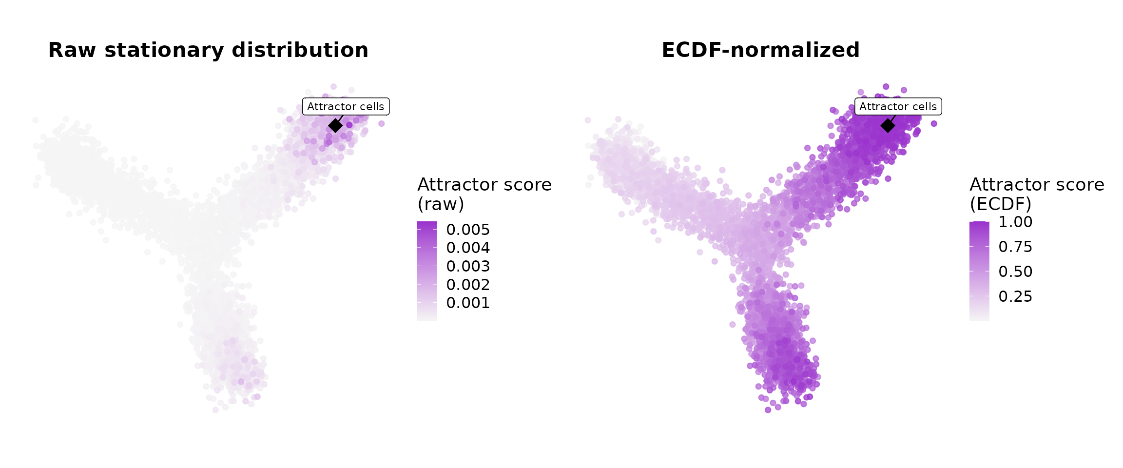

The same cells can be shown as a binary classification — the top 2% of the stationary distribution, flagged as predicted attractor cells:

DimPlot(
    seurat_obj,
    reduction = 'pca',
    group.by  = 'attractor_state',
    cols      = c('Other' = 'lightgrey', 'Attractor' = 'darkorchid3'),
    pt.size   = 1.5
) + coord_equal() + ggtitle('Predicted attractor cells — turquoise, knock-down')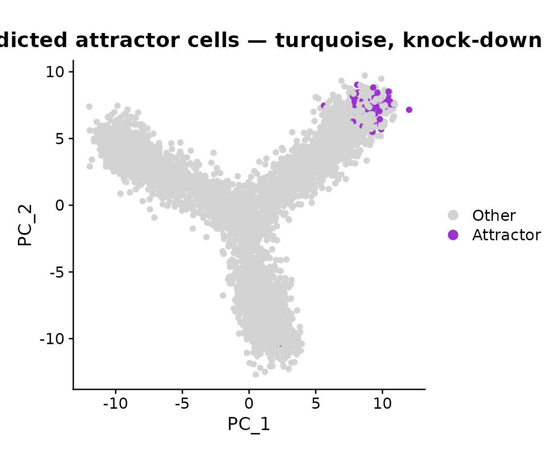

Terminal states on the branches that the perturbation drives cells toward should show the highest attractor scores. After turquoise knock-down, we expect the attractor mass to concentrate at the branch tip that the knock-down promotes, and to shift away from the turquoise-enriched branch.

Markov hitting time (perturbation pseudotime)

PredictPerturbationTime sets up an absorbing Markov chain with the sink cells as absorbing states and computes the expected number of steps each cell needs to reach the sink. This is analogous to RNA velocity pseudotime, but derived from in-silico perturbation transition probabilities. Sink cells receive a “perturbation pseudotime” of 0; cells that never reach the sink within max_iter steps (default 10,000) are flagged as unconverged.

seurat_obj <- PredictPerturbationTime(
    seurat_obj,
    sink_cells = sink_cells,
    perturbation_name = perturb_name,
    graph = 'RNA_snn'
)

Visualize on the embedding with PlotMarkovEmbedding. We pass sink_cells so the absorbing state (B1-1) is marked with a centroid diamond, and we grey out any unconverged cells so they do not distort the color scale:

# cells that hit max_iter are unconverged — grey them out rather than color them
unconverged_cells <- colnames(seurat_obj)[seurat_obj$perturbation_pseudotime >= 10000]

p_pseudotime <- PlotMarkovEmbedding(
    seurat_obj,
    feature           = 'perturbation_pseudotime',
    reduction         = 'pca',
    sink_cells        = sink_cells,
    sink_label        = 'B1-4 (absorbing state)',
    unconverged_cells = unconverged_cells,
    color_scale       = viridis::plasma(256),
    pt_size           = 1.5,
    legend_title      = 'Perturbation \npseudotime',
    title             = 'Turquoise, knock-down'
) + coord_equal()

print(p_pseudotime)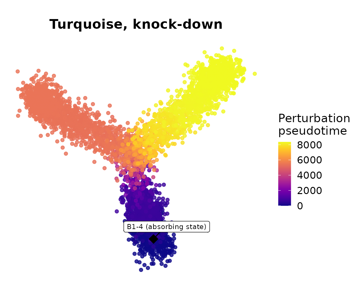

Cells far from the sink in transition probability space will have high pseudotime values. When turquoise is knocked down, cells that would normally move toward the turquoise-enriched branch should instead require many more steps (or move in a different direction) to reach the root. The centroid diamond marks where the clock is anchored: sink cells at B1-1 have pseudotime 0 by definition.

Predicting specific cell fates

PredictFates computes the committor probability, the probability that a random walk starting from each cell will reach a specified target group before leaving the graph. This answers the question: “Given where this cell is, how likely is it to end up in state X?”

In this example, we use this function to calculate the probability that each cell ends up in the B1-4 group.

seurat_obj <- PredictFates(
    seurat_obj,
    perturbation_name = perturb_name,
    graph = 'RNA_snn',
    group.by = 'Group',
    group_name = 'B1-4'
)

We mark the B1-4 target cells with a centroid diamond so their position on the embedding is unambiguous:

fate_target_cells <- colnames(seurat_obj)[seurat_obj$Group == 'B1-4']

p_fates <- PlotMarkovEmbedding(
    seurat_obj,
    feature      = 'forward_fate',
    reduction    = 'pca',
    sink_cells   = fate_target_cells,
    sink_label   = 'B1-4 (fate target)',
    color_scale  = c('whitesmoke', 'darkorchid3'),
    pt_size      = 1.5,
    legend_title = 'Fate probability',
    title        = 'Turquoise, knock-down'
) + coord_equal()

print(p_fates)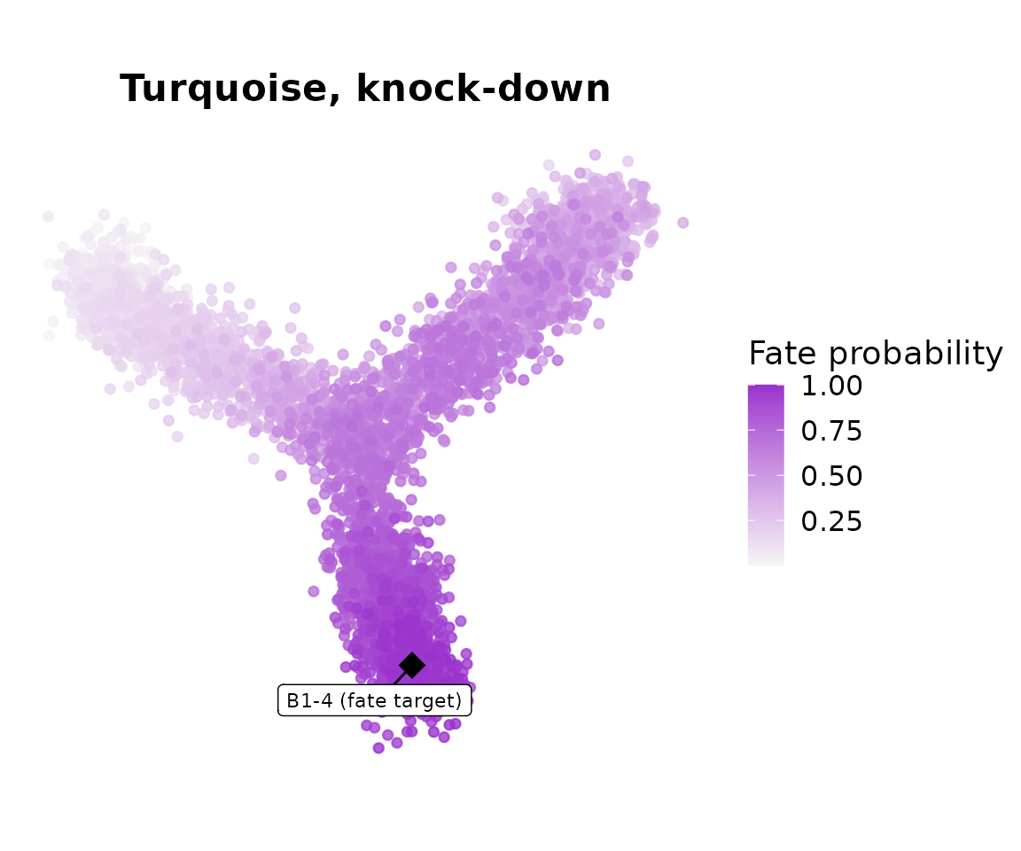

Cells on Branch 1 should have high fate probability toward B1-4. If turquoise drives differentiation along a different branch, knocking it down should not dramatically alter Branch 1 fate probabilities, while fate probabilities toward the turquoise-enriched branch tip should decrease.

Commitment between two states

PredictCommitment computes the committor probability between two specified groups. In general it quantifies how committed each cell is to transitioning from the source state toward the sink state, but the same function could also be used equivalently to study the whether a cell will commit to one of two terminal states.

seurat_obj <- PredictCommitment(
    seurat_obj,
    perturbation_name = perturb_name,
    graph = 'RNA_snn',
    group.by = 'Group',
    source_group = 'B1-4',
    sink_group = 'B3-4'
)

Both boundary populations are marked with labeled centroid diamonds, anchoring the gradient so the reader immediately sees where the 0 and 1 ends lie:

p_commitment <- PlotMarkovEmbedding(
    seurat_obj,
    feature       = 'commitment_score',
    reduction     = 'pca',
    source_cells  = colnames(seurat_obj)[seurat_obj$Group == 'B1-4'],
    sink_cells    = colnames(seurat_obj)[seurat_obj$Group == 'B3-4'],
    source_label  = 'B1-4',
    sink_label    = 'B3-4',
    pt_size       = 1,
    legend_title  = 'Commitment',
    title         = 'Commitment to B1-4 or B3-4'
) + coord_equal() + scale_color_gradientn(
  colors = c(cp["B1-4"], "whitesmoke", "whitesmoke", cp["B3-4"]),
  values = c(0, 0.25, 0.75, 1),
  limits = c(0, 1)
)

print(p_commitment)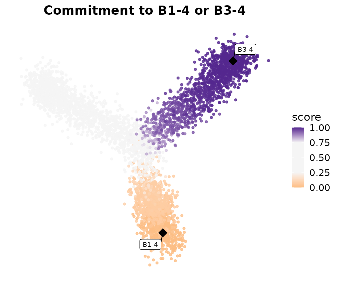

Cells along the Branch 1 trajectory should show a gradient from 0 (at B1-1, the source) to 1 (at B1-4, the sink). Cells on Branches 2 and 3 should have lower commitment scores for this source–sink pair, since their perturbation-driven transitions are not directed toward B1-4.

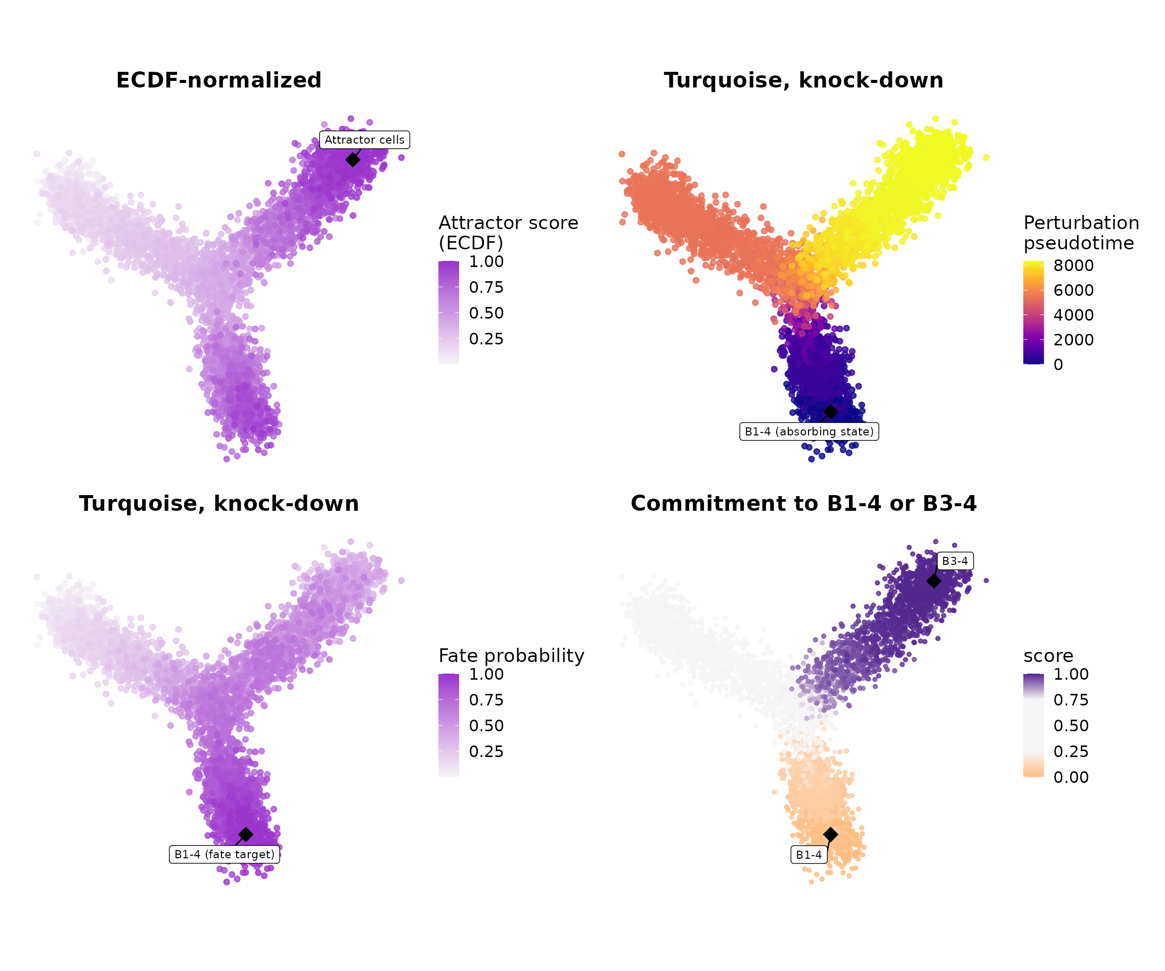
Summary: all four Markov analyses

With all four scores computed, we can display them together in a single 2 × 2 panel:

wrap_plots(
    p_attractors, p_pseudotime,
    p_fates,      p_commitment,
    ncol = 2
)

Alternative visualizations

Individual embedding plots show where each score is high or low across the manifold. compact also includs another visualization function PlotMarkovScatter to examine relationships between predicted cell fate scores or between a score and a biological feature, colored by a grouping variable. Two illustrative comparisons are shown below.

Module eigengene vs. commitment score — turquoise expression should predict commitment to B1-4, since the module is enriched at that branch tip. The dashed reference line at 0.5 marks the threshold above which a cell is more likely to reach B1-4 than to return to B1-1.

PlotMarkovScatter(
    seurat_obj,
    x_feature     = cur_mod,
    y_feature     = 'commitment_score',
    color.by      = 'Group',
    hline         = 0.5,
    x_label       = 'Turquoise module eigengene',
    y_label       = 'Commitment P(B1-4 before B1-1)',
    title         = 'Module expression vs. commitment'
) + scale_color_manual(values=cp)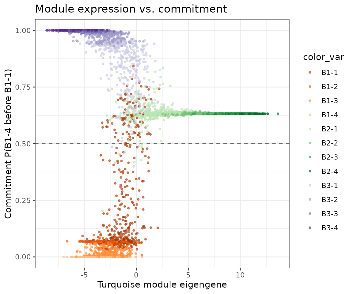

Attractor score vs. perturbation pseudotime — attractor cells are where the random walk converges; they should cluster at low pseudotime values (close to the root sink in transition space) or at particular branch tips depending on the perturbation direction.

PlotMarkovScatter(
    seurat_obj,
    x_feature = 'attractor_score',
    y_feature = 'perturbation_pseudotime',
    color.by  = 'Group',
    x_label   = 'Attractor score',
    y_label   = 'Perturbation pseudotime',
    title     = 'Attractor score vs. pseudotime'
) + scale_color_manual(values=cp)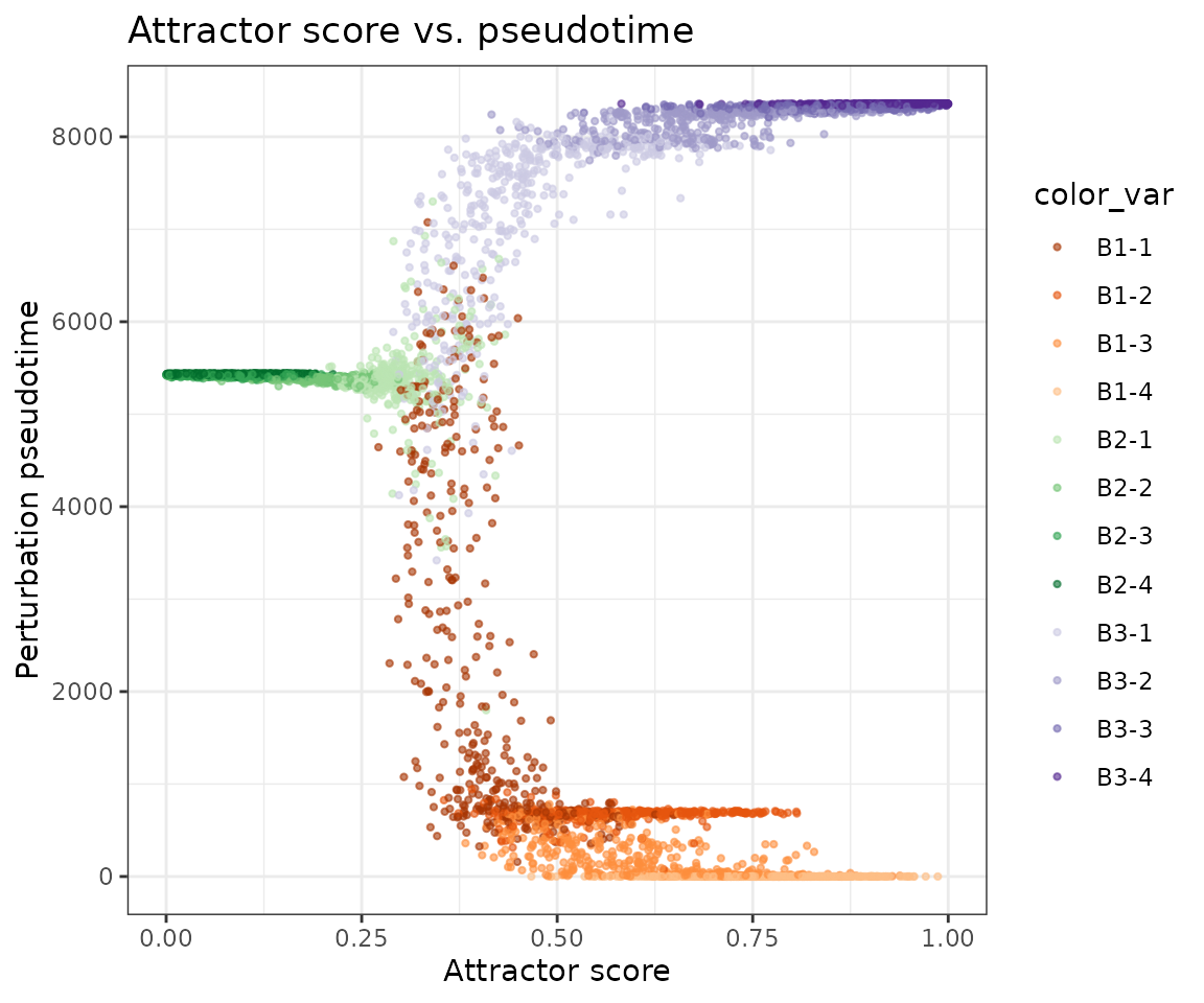

Each branch forms a distinct cluster in this space: cells with high attractor score are either near the root (low pseudotime) or concentrated at branch tips.

---

Summary and next steps

In this tutorial we used compact to perform in-silico module perturbations on a simulated branching trajectory and validated the results against the known ground truth. We:

1. Loaded a pre-processed Seurat object with hdWGCNA co-expression modules already embedded.
2. Built a KNN graph with FindNeighbors to define the local cell neighborhoods.
3. Ran ModulePerturbation to knock down and knock in the turquoise module, producing perturbed expression matrices and transition probability graphs.
4. Verified expression changes with violin plots and PerturbationLog2FC — hub genes showed the largest changes, scaling with kME.
5. Visualized cell-state transitions as vector fields with PlotTransitionVectors — the two directions produced opposite fields as expected.
6. Quantified the local consistency of those transitions with VectorFieldCoherence.
7. Coarse-grained the transition probability matrix to the group level with MacrostateTransitions, reading group-level stability indices and cross-group flow from the Q matrix heatmap.
8. Performed Markov chain analyses to extract pseudotime (PredictPerturbationTime), attractors (PredictAttractors), fate probabilities (PredictFates), and commitment scores (PredictCommitment), visualized with PlotMarkovEmbedding (source/sink overlays, unconverged-cell greying) and PlotMarkovScatter (cross-score relationships).

The same workflow applies directly to real biological datasets. For a tutorial using Alzheimer’s disease microglia or NSCLC data, see the basic tutorial (⚠️ under construction, coming soon).

For transcription factor–based perturbations using TFPerturbation, see the TF perturbation tutorial (coming soon).

Session information (click to expand)

sessionInfo()
#> R version 4.5.3 (2026-03-11)
#> Platform: x86_64-conda-linux-gnu
#> Running under: CentOS Linux 7 (Core)
#> 
#> Matrix products: default
#> BLAS/LAPACK: /home/groups/singlecell/smorabito/.conda/envs/compact_fresh/lib/libopenblasp-r0.3.32.so;  LAPACK version 3.12.0
#> 
#> locale:
#>  [1] LC_CTYPE=en_US.UTF-8       LC_NUMERIC=C              
#>  [3] LC_TIME=en_US.UTF-8        LC_COLLATE=en_US.UTF-8    
#>  [5] LC_MONETARY=en_US.UTF-8    LC_MESSAGES=en_US.UTF-8   
#>  [7] LC_PAPER=en_US.UTF-8       LC_NAME=C                 
#>  [9] LC_ADDRESS=C               LC_TELEPHONE=C            
#> [11] LC_MEASUREMENT=en_US.UTF-8 LC_IDENTIFICATION=C       
#> 
#> time zone: Europe/Madrid
#> tzcode source: system (glibc)
#> 
#> attached base packages:
#> [1] stats4    stats     graphics  grDevices utils     datasets  methods  
#> [8] base     
#> 
#> other attached packages:
#>  [1] ggpubr_0.6.3                future_1.70.0              
#>  [3] compact_0.1.0               hdWGCNA_0.4.11             
#>  [5] enrichR_3.4                 SummarizedExperiment_1.40.0
#>  [7] Biobase_2.70.0              MatrixGenerics_1.22.0      
#>  [9] matrixStats_1.5.0           GenomicRanges_1.62.1       
#> [11] Seqinfo_1.0.0               IRanges_2.44.0             
#> [13] S4Vectors_0.48.0            BiocGenerics_0.56.0        
#> [15] generics_0.1.4              GeneOverlap_1.46.0         
#> [17] UCell_2.14.0                tidygraph_1.3.0            
#> [19] ggraph_2.2.2                igraph_2.3.1               
#> [21] WGCNA_1.74                  fastcluster_1.3.0          
#> [23] dynamicTreeCut_1.63-1       ggrepel_0.9.8              
#> [25] harmony_2.0.2               Rcpp_1.1.1-1.1             
#> [27] RColorBrewer_1.1-3          patchwork_1.3.2            
#> [29] cowplot_1.2.0               lubridate_1.9.5            
#> [31] forcats_1.0.1               stringr_1.6.0              
#> [33] dplyr_1.2.1                 purrr_1.2.2                
#> [35] readr_2.2.0                 tidyr_1.3.2                
#> [37] tibble_3.3.1                ggplot2_4.0.3              
#> [39] tidyverse_2.0.0             Seurat_5.5.0               
#> [41] SeuratObject_5.4.0          sp_2.2-1                   
#> 
#> loaded via a namespace (and not attached):
#>   [1] fs_2.1.0                    spatstat.sparse_3.1-0      
#>   [3] bitops_1.0-9                httr_1.4.8                 
#>   [5] doParallel_1.0.17           tools_4.5.3                
#>   [7] sctransform_0.4.3           backports_1.5.1            
#>   [9] R6_2.6.1                    lazyeval_0.2.3             
#>  [11] uwot_0.2.4                  withr_3.0.2                
#>  [13] gridExtra_2.3               preprocessCore_1.72.0      
#>  [15] progressr_0.19.0            cli_3.6.6                  
#>  [17] textshaping_1.0.5           Cairo_1.7-0                
#>  [19] spatstat.explore_3.8-0      fastDummies_1.7.6          
#>  [21] labeling_0.4.3              sass_0.4.10                
#>  [23] S7_0.2.2                    spatstat.data_3.1-9        
#>  [25] proxy_0.4-29                ggridges_0.5.7             
#>  [27] pbapply_1.7-4               pkgdown_2.2.0              
#>  [29] systemfonts_1.3.2           foreign_0.8-91             
#>  [31] pscl_1.5.9                  parallelly_1.47.0          
#>  [33] WriteXLS_6.8.0              VGAM_1.1-14                
#>  [35] rstudioapi_0.18.0           impute_1.84.0              
#>  [37] gtools_3.9.5                ica_1.0-3                  
#>  [39] spatstat.random_3.4-5       car_3.1-5                  
#>  [41] Matrix_1.7-5                ggbeeswarm_0.7.3           
#>  [43] abind_1.4-8                 lifecycle_1.0.5            
#>  [45] yaml_2.3.12                 carData_3.0-6              
#>  [47] gplots_3.3.0                SparseArray_1.10.8         
#>  [49] Rtsne_0.17                  grid_4.5.3                 
#>  [51] promises_1.5.0              miniUI_0.1.2               
#>  [53] lattice_0.22-9              pillar_1.11.1              
#>  [55] knitr_1.51                  rjson_0.2.23               
#>  [57] xgboost_3.2.0.1             future.apply_1.20.2        
#>  [59] codetools_0.2-20            glue_1.8.1                 
#>  [61] spatstat.univar_3.1-7       data.table_1.18.2.1        
#>  [63] vctrs_0.7.3                 png_0.1-9                  
#>  [65] spam_2.11-3                 gtable_0.3.6               
#>  [67] cachem_1.1.0                xfun_0.57                  
#>  [69] S4Arrays_1.10.1             mime_0.13                  
#>  [71] survival_3.8-6              SingleCellExperiment_1.32.0
#>  [73] iterators_1.0.14            fitdistrplus_1.2-6         
#>  [75] ROCR_1.0-12                 nlme_3.1-169               
#>  [77] SHAPforxgboost_0.2.0        RcppAnnoy_0.0.23           
#>  [79] bslib_0.10.0                irlba_2.3.7                
#>  [81] vipor_0.4.7                 KernSmooth_2.23-26         
#>  [83] otel_0.2.0                  rpart_4.1.27               
#>  [85] colorspace_2.1-2            Hmisc_5.2-5                
#>  [87] nnet_7.3-20                 ggrastr_1.0.2              
#>  [89] tidyselect_1.2.1            compiler_4.5.3             
#>  [91] curl_7.1.0                  htmlTable_2.5.0            
#>  [93] BiocNeighbors_2.4.0         desc_1.4.3                 
#>  [95] DelayedArray_0.36.0         plotly_4.12.0              
#>  [97] checkmate_2.3.4             scales_1.4.0               
#>  [99] caTools_1.18.3              lmtest_0.9-40              
#> [101] digest_0.6.39               goftest_1.2-3              
#> [103] spatstat.utils_3.2-2        rmarkdown_2.31             
#> [105] XVector_0.50.0              htmltools_0.5.9            
#> [107] pkgconfig_2.0.3             base64enc_0.1-6            
#> [109] fastmap_1.2.0               rlang_1.2.0                
#> [111] htmlwidgets_1.6.4           BBmisc_1.13.1              
#> [113] shiny_1.13.0                farver_2.1.2               
#> [115] jquerylib_0.1.4             zoo_1.8-15                 
#> [117] jsonlite_2.0.0              BiocParallel_1.44.0        
#> [119] magrittr_2.0.5              Formula_1.2-5              
#> [121] dotCall64_1.2               viridis_0.6.5              
#> [123] reticulate_1.46.0           stringi_1.8.7              
#> [125] MASS_7.3-65                 plyr_1.8.9                 
#> [127] parallel_4.5.3              listenv_0.10.1             
#> [129] deldir_2.0-4                graphlayouts_1.2.3         
#> [131] splines_4.5.3               tensor_1.5.1               
#> [133] hms_1.1.4                   rdist_0.0.5                
#> [135] spatstat.geom_3.7-3         ggsignif_0.6.4             
#> [137] RcppHNSW_0.6.0              reshape2_1.4.5             
#> [139] evaluate_1.0.5              tester_0.3.0               
#> [141] tzdb_0.5.0                  foreach_1.5.2              
#> [143] tweenr_2.0.3                httpuv_1.6.17              
#> [145] RANN_2.6.2                  polyclip_1.10-7            
#> [147] scattermore_1.2             ggforce_0.5.0              
#> [149] broom_1.0.12                xtable_1.8-8               
#> [151] RSpectra_0.16-2             rstatix_0.7.3              
#> [153] later_1.4.8                 viridisLite_0.4.3          
#> [155] ragg_1.5.2                  beeswarm_0.4.0             
#> [157] memoise_2.0.1               cluster_2.1.8.2            
#> [159] timechange_0.4.0            globals_0.19.1