Compiled: 07-06-2024
Source: vignettes/basic_tutorial.Rmd
Introduction
This tutorial covers the basics of using hdWGCNA to perform co-expression network analysis on single-cell data. Here, we start with a processed single-nucleus RNA-seq (snRNA-seq) dataset of human cortical samples from this publication. This dataset has already been fully processed using a standard single-cell transcritpomics analysis pipeline such as Seurat or Scanpy. If you would like to follow this tutorial using your own dataset, you first need to satisfy the following prerequisites:
- A single-cell or single-nucleus transcriptomics dataset in Seurat format.
- Normalize the gene expression matrix NormalizeData.
- Identify highly variable genes VariableFeatures.
- Scale the normalized expression data ScaleData
- Perform dimensionality reduction RunPCA and batch correction if needed RunHarmony.
- Non-linear dimensionality reduction RunUMAP for visualizations.
- Group cells into clusters (FindNeighbors and FindClusters).
An example of running the prerequisite data processing steps can be found in the Seurat Guided Clustering Tutorial.
Additionally, there are a lot of WGCNA-specific terminology and acronyms, which are all clarified in this table.
Important note: We do not re-generate these tutorial figures after each update of hdWGCNA, so the figures that you generate will be slightly different than what are shown here if you are following along with the same dataset.
Download the tutorial data
For the purpose of this tutorial, we provide a processed Seurat object of the control human brains from the Zhou et al 2020 study.
Please download the file Zhou_2020_control.rds from this
Google
Drive link.
Load the dataset and required libraries
First we will load the single-cell dataset and the required R libraries for this tutorial.
# single-cell analysis package
library(Seurat)

# plotting and data science packages
library(tidyverse)
library(cowplot)
library(patchwork)

# co-expression network analysis packages:
library(WGCNA)
library(hdWGCNA)

# using the cowplot theme for ggplot
theme_set(theme_cowplot())

# set random seed for reproducibility
set.seed(12345)

# optionally enable multithreading
enableWGCNAThreads(nThreads = 8)

# load the Zhou et al snRNA-seq dataset
seurat_obj <- readRDS('Zhou_2020_control.rds')
This Seurat object was originally created using Seruat v4. If you are using Seurat v5, please run this additional command.
seurat_obj <- SeuratObject::UpdateSeuratObject(seurat_obj)Here we will plot the UMAP colored by cell type just to check that we have loaded the data correctly, and to make sure that we have grouped cells into clusters and cell types.
p <- DimPlot(seurat_obj, group.by='cell_type', label=TRUE) +
   umap_theme() + ggtitle('Zhou et al Control Cortex') + NoLegend()

p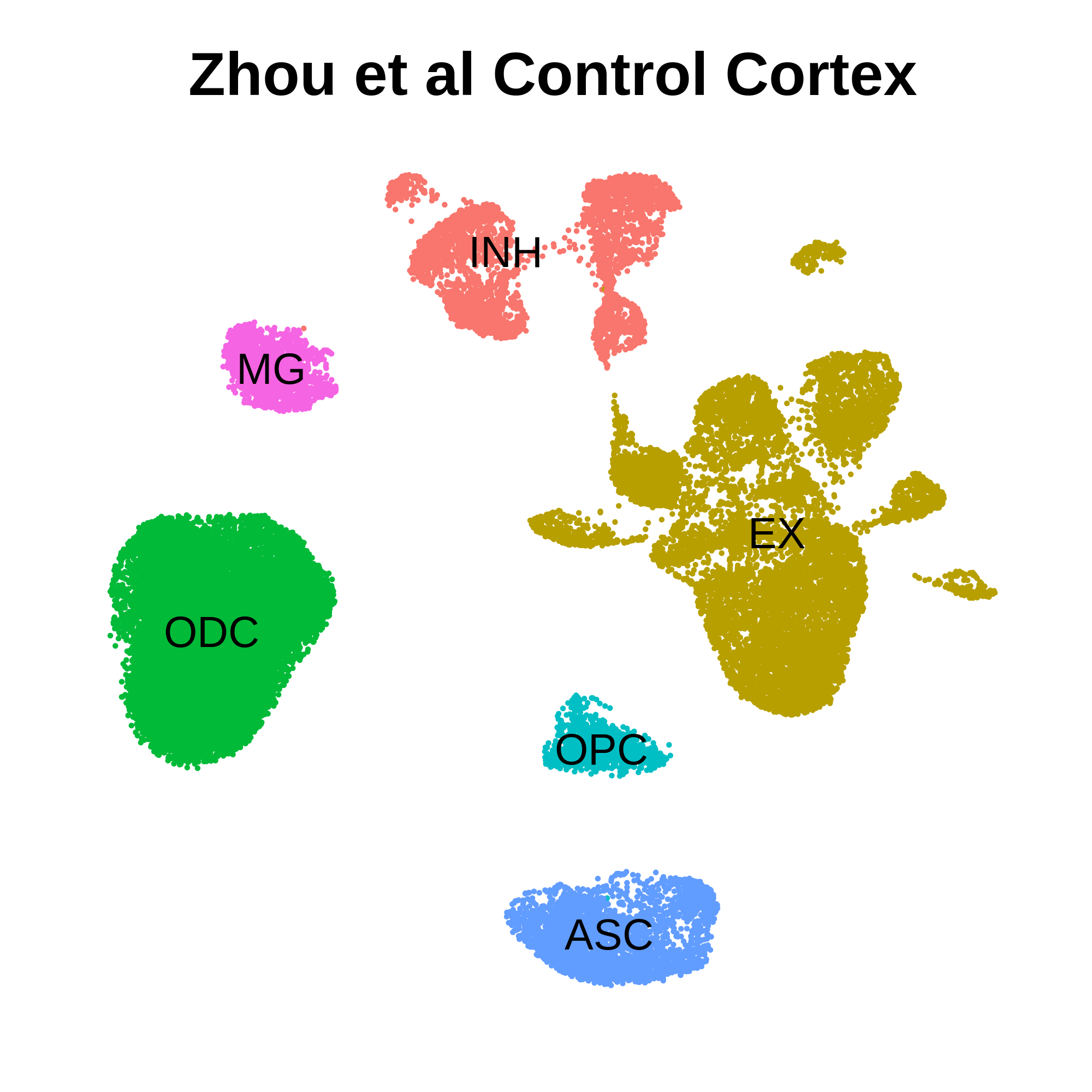
Set up Seurat object for WGCNA
Before running hdWGCNA, we first have to set up the Seurat object.
Most of the information computed by hdWGCNA is stored in the Seurat
object’s @misc slot, and all of this information can be
retrieved by various getter and setter functions. A single Seurat object
can hold multiple hdWGCNA experiments, for example representing
different cell types in the same single-cell dataset. Notably, since we
consider hdWGCNA to be a downstream data analysis step, we
do not support subsetting the Seurat object after
SetupForWGCNA has been run.
Here we will set up the Seurat object using the
SetupForWGCNA function, specifying the name of the hdWGNCA
experiment. This function also selects the genes that will be used for
WGCNA. The user can select genes using three different approaches using
the gene_select parameter:
-
variable: use the genes stored in the Seurat object’sVariableFeatures. -
fraction: use genes that are expressed in a certain fraction of cells for in the whole dataset or in each group of cells, specified bygroup.by. -
custom: use genes that are specified in a custom list.
In this example, we will select genes that are expressed in at least 5% of cells in this dataset, and we will name our hdWGCNA experiment “tutorial”.
seurat_obj <- SetupForWGCNA(
  seurat_obj,
  gene_select = "fraction", # the gene selection approach
  fraction = 0.05, # fraction of cells that a gene needs to be expressed in order to be included
  wgcna_name = "tutorial" # the name of the hdWGCNA experiment
)
Construct metacells
After we have set up our Seurat object, the first step in running the hdWGCNA pipeine in hdWGCNA is to construct metacells from the single-cell dataset. Briefly, metacells are aggregates of small groups of similar cells originating from the same biological sample of origin. The k-Nearest Neighbors (KNN) algorithm is used to identify groups of similar cells to aggregate, and then the average or summed expression of these cells is computed, thus yielding a metacell gene expression matrix. The sparsity of the metacell expression matrix is considerably reduced when compared to the original expression matrix, and therefore it is preferable to use. We were originally motivated to use metacells in place of the original single cells because correlation network approaches such as WGCNA are sensitive to data sparsity.
hdWGCNA includes a function MetacellsByGroups to
construct metacell expression matrices given a single-cell dataset. This
function constructs a new Seurat object for the metacell dataset which
is stored internally in the hdWGCNA experiment. The
group.by parameter determines which groups metacells will
be constructed in. We only want to construct metacells from cells that
came from the same biological sample of origin, so it is critical to
pass that information to hdWGCNA via the group.by
parameter. Additionally, we usually construct metacells for each cell
type separately. Thus, in this example, we are grouping by
Sample and cell_type to achieve the desired
result.
The number of cells to be aggregated k should be tuned
based on the size of the input dataset, in general a lower number for
k can be used for small datasets. We generally use
k values between 20 and 75. The dataset used for this
tutorial has 40,039 cells, ranging from 890 to 8,188 in each biological
sample, and here we used k=25. The amount of allowable
overlap between metacells can be tuned using the max_shared
argument. There should be a range of K values that are suitable for
reducing the sparsity while retaining cellular heterogeneity for a given
dataset, rather than a single optimal value.
Note: we have found that the metacell
aggregation approach does not yield good results for extremely
underrepresented cell types. For example, in this dataset, the brain
vascular cells (pericytes and endothelial cells) were the least
represented, and we have excluded them from this analysis.
MetacellsByGroups has a parameter min_cells to
exclude groups that are smaller than a specified number of cells. Errors
are likely to arise if the selected value for min_cells is
too low.
Here we construct metacells and normalize the resulting expression matrix using the following code:
# construct metacells  in each group
seurat_obj <- MetacellsByGroups(
  seurat_obj = seurat_obj,
  group.by = c("cell_type", "Sample"), # specify the columns in seurat_obj@meta.data to group by
  reduction = 'harmony', # select the dimensionality reduction to perform KNN on
  k = 25, # nearest-neighbors parameter
  max_shared = 10, # maximum number of shared cells between two metacells
  ident.group = 'cell_type' # set the Idents of the metacell seurat object
)

# normalize metacell expression matrix:
seurat_obj <- NormalizeMetacells(seurat_obj)
Optional: Process the Metacell Seurat Object
Since we store the Metacell expression information as its own Seurat
object, we can run Seurat functions on the metacell data. We can get the
metacell object from the hdWGCNA experiment using
GetMetacellObject.
metacell_obj <- GetMetacellObject(seurat_obj)Additionally, we have included a few wrapper functions to apply the Seurat workflow to the metacell object within the hdWGCNA experiment. Here we apply these wrapper functions to process the metacell object and visualize the aggregated expression profiles in two dimensions with UMAP.
seurat_obj <- NormalizeMetacells(seurat_obj)
seurat_obj <- ScaleMetacells(seurat_obj, features=VariableFeatures(seurat_obj))
seurat_obj <- RunPCAMetacells(seurat_obj, features=VariableFeatures(seurat_obj))
seurat_obj <- RunHarmonyMetacells(seurat_obj, group.by.vars='Sample')
seurat_obj <- RunUMAPMetacells(seurat_obj, reduction='harmony', dims=1:15)


p1 <- DimPlotMetacells(seurat_obj, group.by='cell_type') + umap_theme() + ggtitle("Cell Type")
p2 <- DimPlotMetacells(seurat_obj, group.by='Sample') + umap_theme() + ggtitle("Sample")

p1 | p2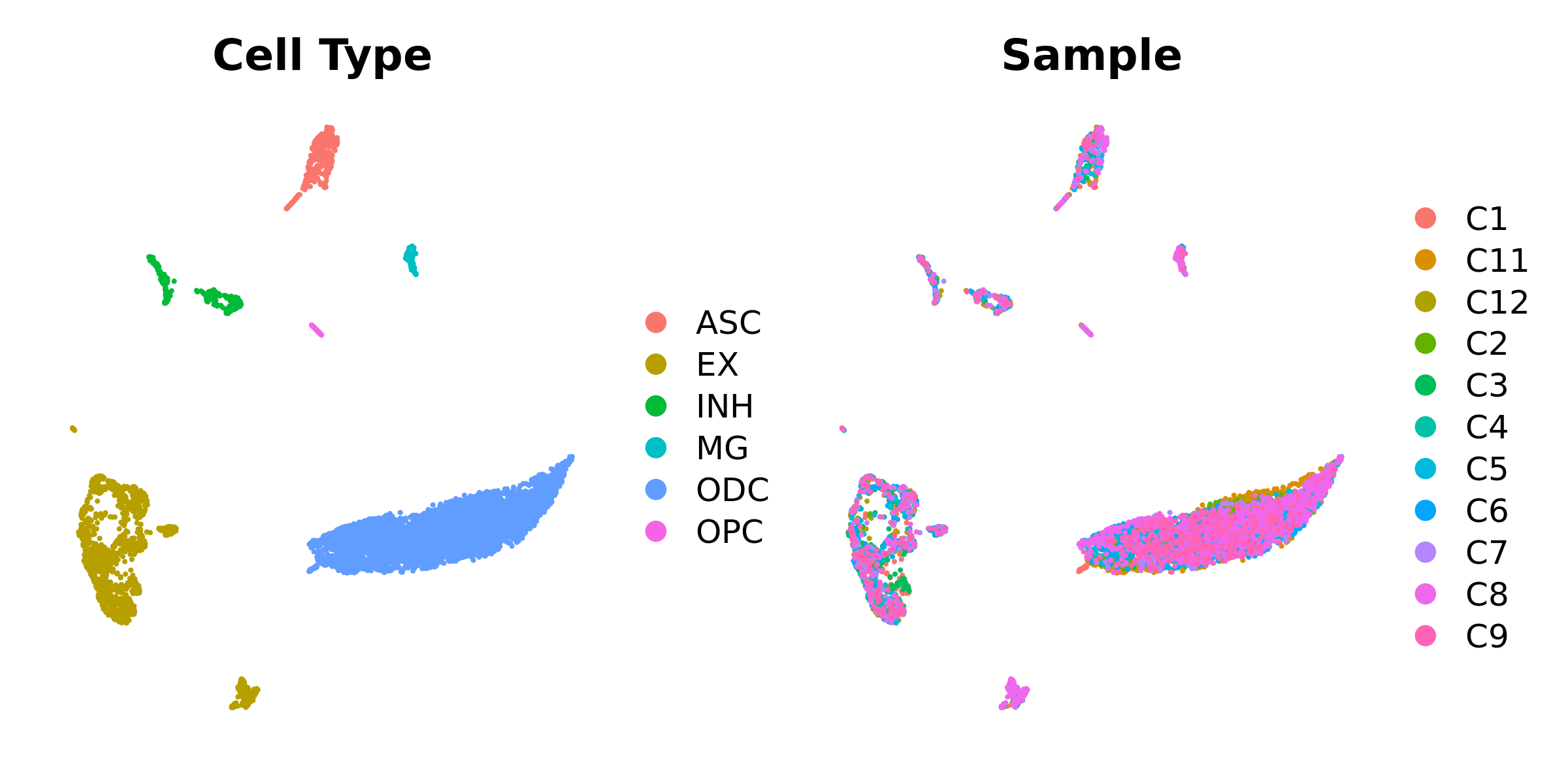
Co-expression network analysis
In this section we discuss how to perform co-expression network analysis with hdWGNCA on the inhibitory neuron (INH) cells in our example dataset.
Set up the expression matrix
Here we specify the expression matrix that we will use for network
analysis. Since We only want to include the inhibitory neurons, so we
have to subset our expression data prior to constructing the network.
hdWGCNA includes the SetDatExpr function to store the
transposed expression matrix for a given group of cells that will be
used for downstream network analysis. The metacell expression matrix is
used by default (use_metacells=TRUE), but hdWGCNA does
allow for the single-cell expression matrix to be used if desired.. This
function allows the user to specify which slot/layer to take the
expression matrix from, for example if the user wanted to apply SCTransform
normalization instead of NormalizeData.
seurat_obj <- SetDatExpr(
  seurat_obj,
  group_name = "INH", # the name of the group of interest in the group.by column
  group.by='cell_type', # the metadata column containing the cell type info. This same column should have also been used in MetacellsByGroups
  assay = 'RNA', # using RNA assay
  layer = 'data' # using normalized data
)
Selecting more than one group
Suppose that you want to perform co-expression network analysis on
more than one cell type or cluster simultaneously.
SetDatExpr can be run with slighly different settings to
achieve the desired result by passing a character vector to the
group_name parameter.
seurat_obj <- SetDatExpr(
  seurat_obj,
  group_name = c("INH", "EX"),
  group.by='cell_type'
)
Select soft-power threshold
Next we will select the “soft power threshold”. This is an extremely important step in the hdWGNCA pipleine (and for vanilla WGCNA). hdWGCNA constructs a gene-gene correlation adjacency matrix to infer co-expression relationships between genes. The correlations are raised to a power to reduce the amount of noise present in the correlation matrix, thereby retaining the strong connections and removing the weak connections. Therefore, it is critical to determine a proper value for the soft power threshold.
We include a function TestSoftPowers to perform a
parameter sweep for different soft power thresholds. This function helps
us to guide our choice in a soft power threshold for constructing the
co-expression network by inspecting the resulting network topology for
different power values. The co-expression network should have a scale-free
topology, therefore the TestSoftPowers function models
how closely the co-expression network resembles a scale-free graph at
different soft power thresholds. Furthermore, we include a function
PlotSoftPowers to visualize the results of the parameter
sweep.
The following code performs the parameter sweep and outputs a summary figure.
# Test different soft powers:
seurat_obj <- TestSoftPowers(
  seurat_obj,
  networkType = 'signed' # you can also use "unsigned" or "signed hybrid"
)

# plot the results:
plot_list <- PlotSoftPowers(seurat_obj)

# assemble with patchwork
wrap_plots(plot_list, ncol=2)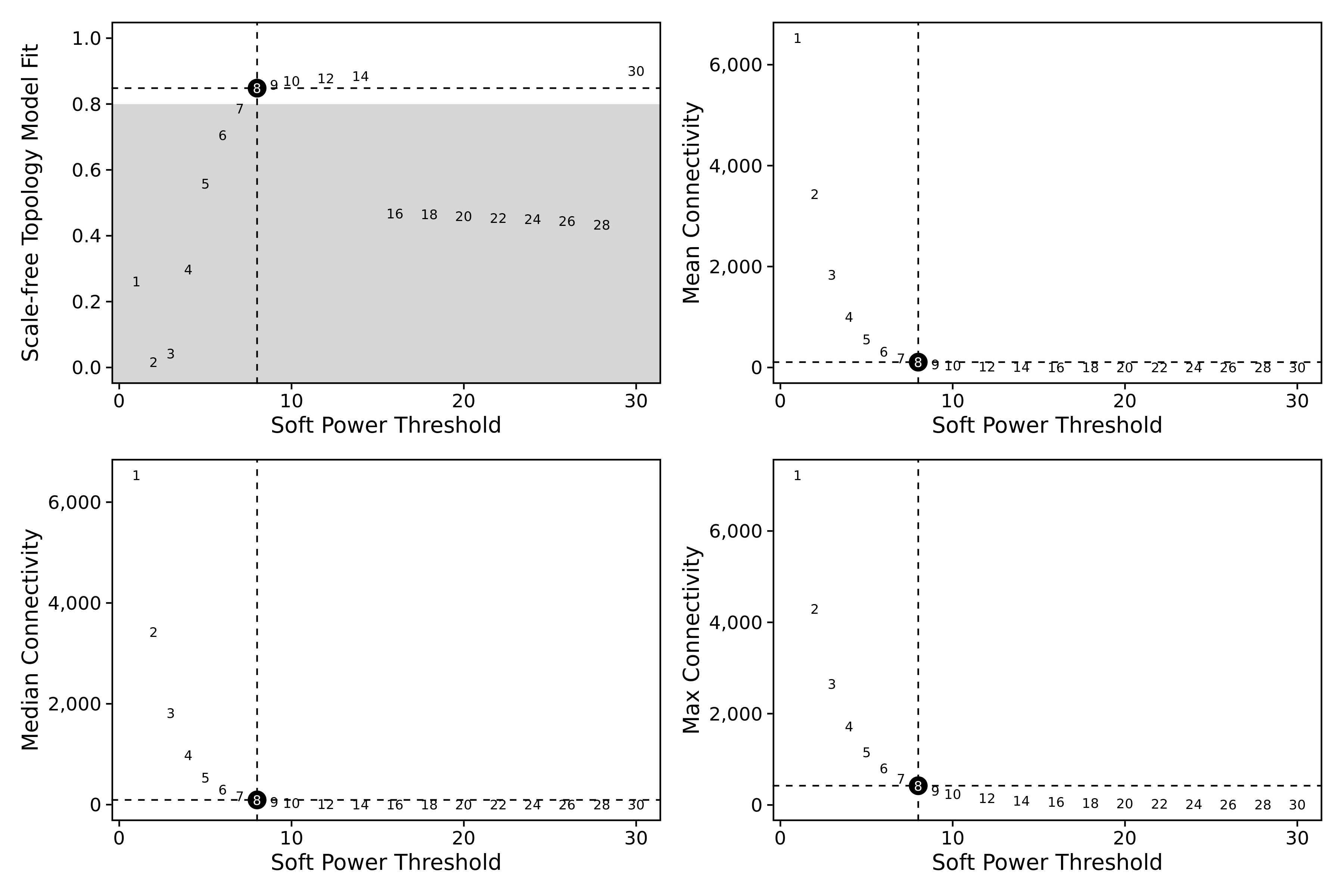
The general guidance for WGCNA and hdWGCNA is to pick the lowest soft
power threshold that has a Scale Free Topology Model Fit greater than or
equal to 0.8, so in this case we would select our soft power threshold
as 9. Later on, the ConstructNetwork will automatically
select the soft power threshold if the user does not provide one.
Tthe output table from the parameter sweep is stored in the hdWGCNA
experiment and can be accessed using the GetPowerTable
function for further inspection:
power_table <- GetPowerTable(seurat_obj)
head(power_table)
Output
  Power   SFT.R.sq     slope truncated.R.sq   mean.k. median.k.    max.k.
1     1 0.26110351 11.889729      0.9546294 6525.7417 6532.2923 7219.7053
2     2 0.01631495  1.375111      0.9935408 3434.0090 3421.8601 4293.1289
3     3 0.04178826 -1.487314      0.9784280 1840.1686 1817.2352 2651.0575
4     4 0.29769630 -3.249674      0.9588046 1003.7962  978.3657 1719.7194
5     5 0.55846894 -4.060086      0.9617106  557.3639  533.2201 1157.0353
6     6 0.70513240 -4.195496      0.9696135  315.0681  295.1368  804.1011
Construct co-expression network
We now have everything that we need to construct our co-expression
network. Here we use the hdWGCNA function ConstructNetwork,
which calls the WGCNA function blockwiseConsensusModules
under the hood. This function has quite a few parameters to play with if
you are an advanced user, but we have selected default parameters that
work well with many single-cell datasets. The parameters for
blockwiseConsensusModules can be passed directly to
ConstructNetwork with the same parameter names.
The following code construtcts the co-expression network using the soft power threshold selected above:
# construct co-expression network:
seurat_obj <- ConstructNetwork(
  seurat_obj,
  tom_name = 'INH' # name of the topoligical overlap matrix written to disk
)
hdWGCNA also includes a function PlotDendrogram to
visualize the WGCNA dendrogram, a common visualization to show the
different co-expression modules resulting from the network analysis.
Each leaf on the dendrogram represents a single gene, and the color at
the bottom indicates the co-expression module assignment.
Importantly, the “grey” module consists of genes that were not grouped into any co-expression module. The grey module should be ignored for all downstream analysis and interpretation.
PlotDendrogram(seurat_obj, main='INH hdWGCNA Dendrogram')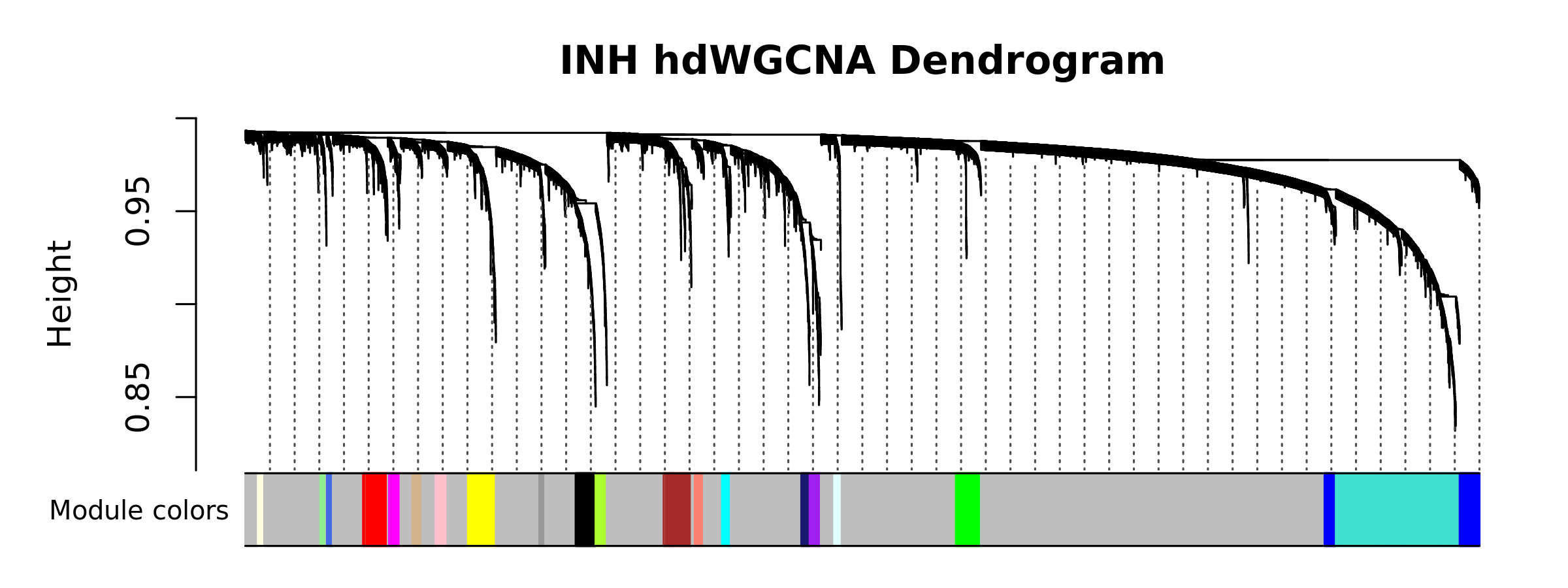
Optional: inspect the topoligcal overlap matrix (TOM)
hdWGCNA represents the co-expression network as a topoligcal overlap
matrix (TOM). This is a square matrix of genes by genes, where each
value is the topoligcal overlap between the genes. The TOM is written to
the disk when running ConstructNetwork, and we can load it
into R using the GetTOM function. Advanced users may wish
to inspect the TOM for custom downstream analyses.
TOM <- GetTOM(seurat_obj)Module Eigengenes and Connectivity
In this section we will cover how to compute module eigengenes in single cells, and how to compute the eigengene-based connectivity for each gene.
Compute harmonized module eigengenes
Module Eigengenes (MEs) are a commonly used metric to summarize the gene expression profile of an entire co-expression module. Briefly, module eigengenes are computed by performing principal component analysis (PCA) on the subset of the gene expression matrix comprising each module. The first PC of each of these PCA matrices are the MEs.
Dimensionality reduction techniques are a very hot topic in single-cell genomics. It is well known that technical artifacts can muddy the analysis of single-cell datasets, and over the years there have been many methods that aim to reduce the effects of these artifacts. Therefore it stands to reason that MEs would be subject to these technical artifacts as well, and hdWGCNA seeks to alleviate these effects.
hdWGCNA includes a function ModuleEigengenes to compute
module eigengenes in single cells. Additionally, we allow the user to
apply Harmony batch correction to the MEs, yielding harmonized
module eigengenes (hMEs). The following code performs the
module eigengene computation harmonizing by the Sample of origin using
the group.by.vars parameter.
# need to run ScaleData first or else harmony throws an error:
#seurat_obj <- ScaleData(seurat_obj, features=VariableFeatures(seurat_obj))

# compute all MEs in the full single-cell dataset
seurat_obj <- ModuleEigengenes(
 seurat_obj,
 group.by.vars="Sample"
)
The ME matrices are stored as a matrix where each row is a cell and
each column is a module. This matrix can be extracted from the Seurat
object using the GetMEs function, which retrieves the
hMEs by default.
Compute module connectivity
In co-expression network analysis, we often want to focus on the “hub
genes”, those which are highly connected within each module. Therefore
we wish to determine the eigengene-based connectivity, also
known as kME, of each gene. hdWGCNA includes the
ModuleConnectivity to compute the kME values in
the full single-cell dataset, rather than the metacell dataset. This
function essentially computes pairwise correlations between genes and
module eigengenes. kME can be computed for all cells in the dataset, but
we recommend computing kME in the cell type or group that was previously
used to run ConstructNetwork.
# compute eigengene-based connectivity (kME):
seurat_obj <- ModuleConnectivity(
  seurat_obj,
  group.by = 'cell_type', group_name = 'INH'
)
For convenience, we re-name the hdWGCNA modules to indicate that they are from the inhibitory neuron group. More information about renaming modules can be found in the module customization tutorial.
# rename the modules
seurat_obj <- ResetModuleNames(
  seurat_obj,
  new_name = "INH-M"
)
We can visualize the genes in each module ranked by kME using the
PlotKMEs function.
# plot genes ranked by kME for each module
p <- PlotKMEs(seurat_obj, ncol=5)

p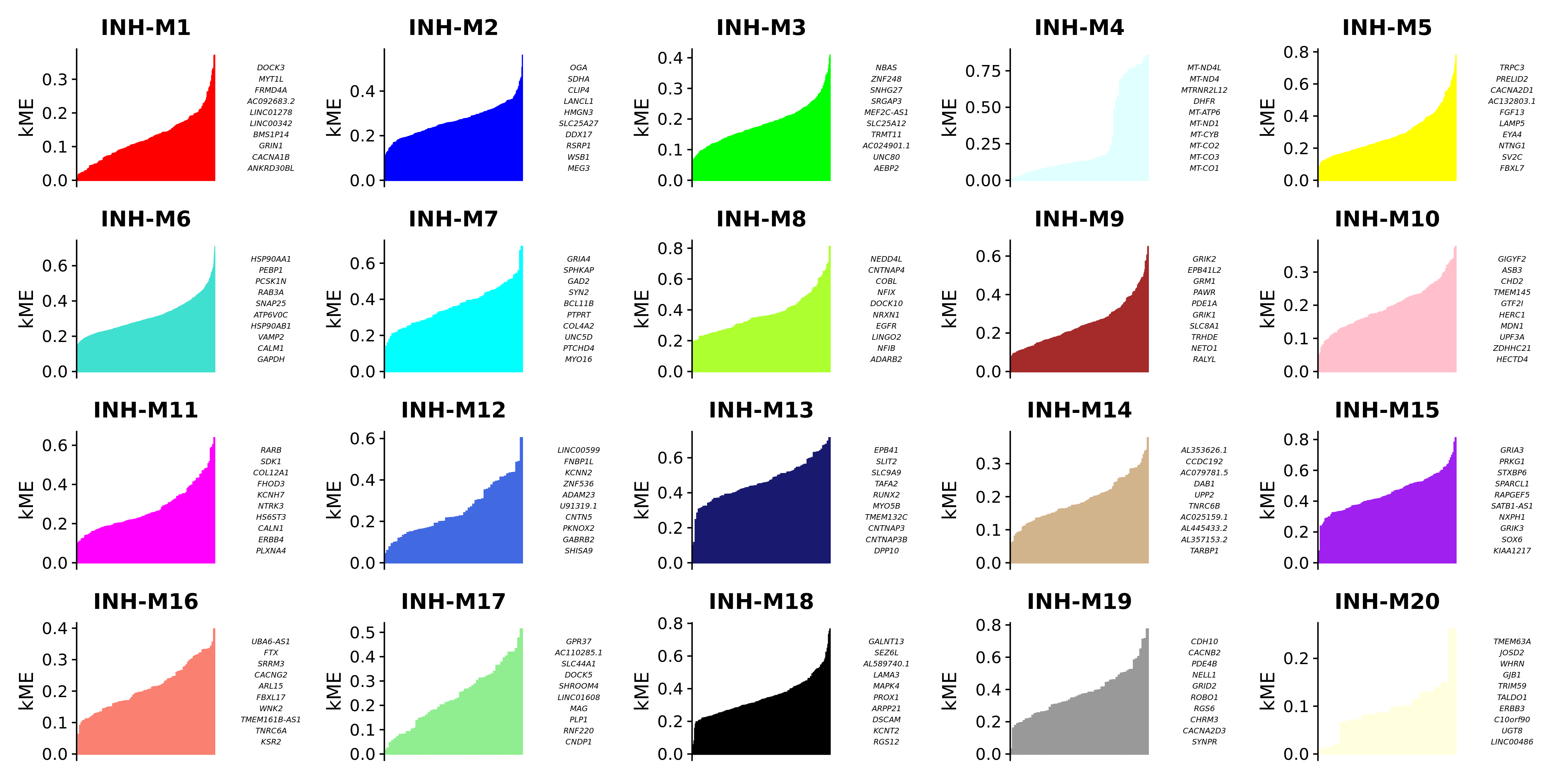
Getting the module assignment table
hdWGCNA allows for easy access of the module assignment table using
the GetModules function. This table consists of three
columns: gene_name stores the gene’s symbol or ID,
module stores the gene’s module assignment, and
color stores a color mapping for each module, which is used
in many downstream plotting steps. If ModuleConnectivity
has been called on this hdWGCNA experiment, this table will have
additional columns for the kME of each module.
# get the module assignment table:
modules <- GetModules(seurat_obj) %>% subset(module != 'grey')

# show the first 6 columns:
head(modules[,1:6])
Output
          gene_name module     color   kME_grey  kME_INH-M1 kME_INH-M2
LINC01409 LINC01409 INH-M1       red 0.06422496  0.14206189 0.02146438
INTS11       INTS11 INH-M2      blue 0.19569750  0.04996486 0.22687525
CCNL2         CCNL2 INH-M3     green 0.21124081  0.04668528 0.20013727
GNB1           GNB1 INH-M4 lightcyan 0.24093763  0.03203763 0.20114899
TNFRSF14   TNFRSF14 INH-M5    yellow 0.01315166  0.02388175 0.02342308
TPRG1L       TPRG1L INH-M6 turquoise 0.10138479 -0.05137751 0.12394048
A table of the top N hub genes sorted by kME can be extracted using
the GetHubGenes function.
# get hub genes
hub_df <- GetHubGenes(seurat_obj, n_hubs = 10)

head(hub_df)
Output
 gene_name module       kME
1 ANKRD30BL INH-M1 0.3711414
2   CACNA1B INH-M1 0.3694937
3     GRIN1 INH-M1 0.3318094
4   BMS1P14 INH-M1 0.3304103
5 LINC00342 INH-M1 0.3252982
6 LINC01278 INH-M1 0.3100343
This wraps up the critical analysis steps for hdWGCNA, so remember to save your output.
saveRDS(seurat_obj, file='hdWGCNA_object.rds')Compute hub gene signature scores
Gene scoring analysis is a popular method in single-cell
transcriptomics for computing a score for the overall signature of a set
of genes. We can use these methods as alternatives to module eigengenes.
hdWGCNA includes the function ModuleExprScore to compute
gene scores for a give number of genes for each module, using either the
UCell or Seurat algorithm.
# compute gene scoring for the top 25 hub genes by kME for each module
# with UCell method
library(UCell)
seurat_obj <- ModuleExprScore(
  seurat_obj,
  n_genes = 25,
  method='UCell'
)
Basic Visualization
Here we showcase some of the basic visualization capabilities of hdWGCNA, and we demonstrate how to use some of Seurat’s built-in plotting tools to visualize our hdWGCNA results. Note that we have a separate tutorial for visualization of the hdWGCNA networks.
Module Feature Plots
FeaturePlot
is a commonly used Seurat visualization to show a feature of interest
directly on the dimensionality reduction. hdWGCNA includes the
ModuleFeaturePlot function to consruct FeaturePlots for
each co-expression module colored by each module’s uniquely assigned
color.
# make a featureplot of hMEs for each module
plot_list <- ModuleFeaturePlot(
  seurat_obj,
  features='hMEs', # plot the hMEs
  order=TRUE # order so the points with highest hMEs are on top
)

# stitch together with patchwork
wrap_plots(plot_list, ncol=6)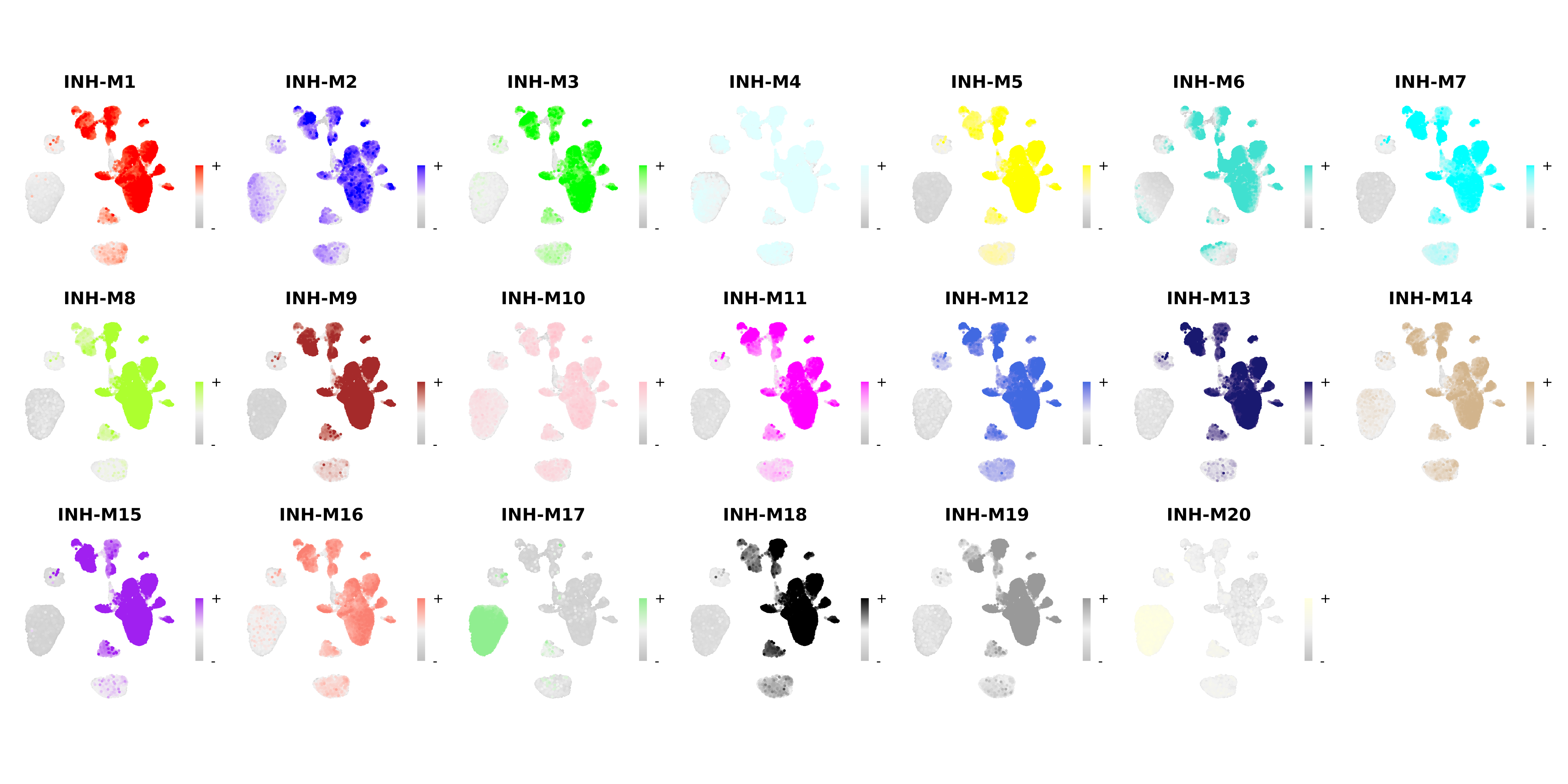
We can also plot the hub gene signature score using the same function:
# make a featureplot of hub scores for each module
plot_list <- ModuleFeaturePlot(
  seurat_obj,
  features='scores', # plot the hub gene scores
  order='shuffle', # order so cells are shuffled
  ucell = TRUE # depending on Seurat vs UCell for gene scoring
)

# stitch together with patchwork
wrap_plots(plot_list, ncol=6)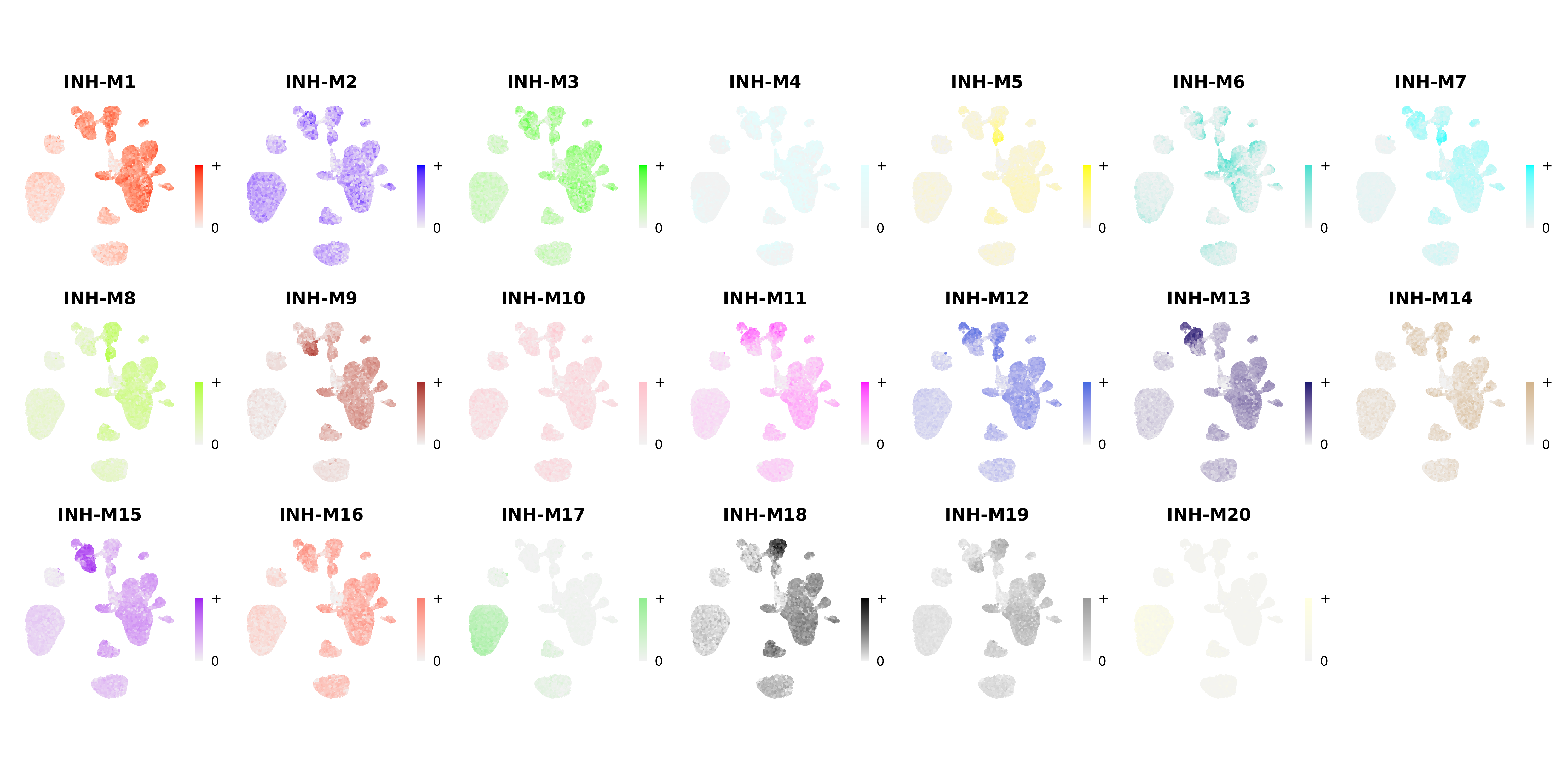
We can also use a radar plot to visualize the relative expression
level of each module across different cell groupings. Here we use the
function ModuleRadarPlot to visualize the expression of
these modules in the INH subclusters.
seurat_obj$cluster <- do.call(rbind, strsplit(as.character(seurat_obj$annotation), ' '))[,1]

ModuleRadarPlot(
  seurat_obj,
  group.by = 'cluster',
  barcodes = seurat_obj@meta.data %>% subset(cell_type == 'INH') %>% rownames(),
  axis.label.size=4,
  grid.label.size=4
)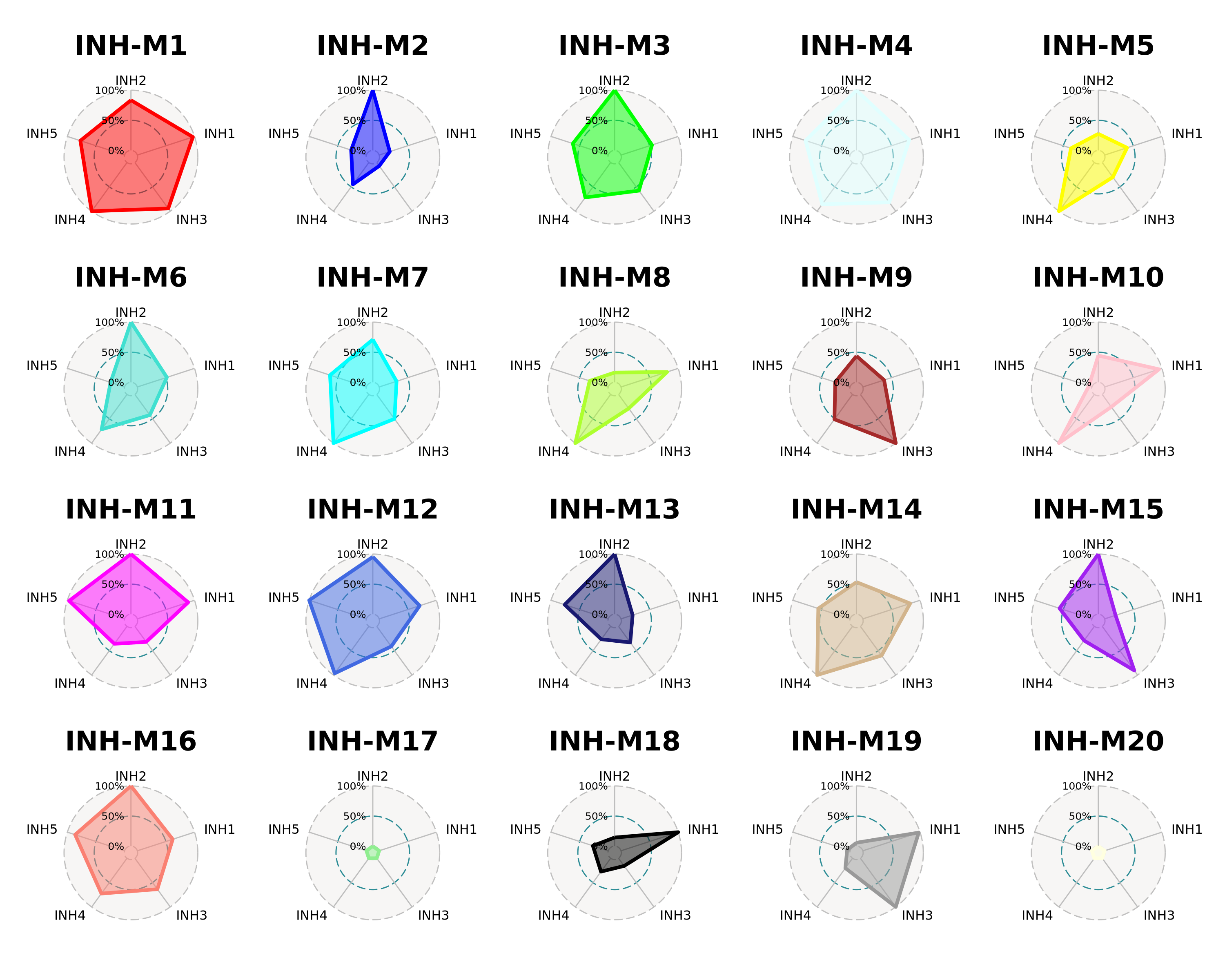
Here we can easily visualize which modules are shared across different INH subtypes, like module INH-M1, as well as modules that are expressed more specifically in one subtype like module INH-M18. For this type of plot we do not recommend trying to visualize too many cell groups at once.
Expand to see Module Correlogram
hdWGCNA includes the ModuleCorrelogram function to
visualize the correlation between each module based on their hMEs, MEs,
or hub gene scores using the R package corrplot.
# plot module correlagram
ModuleCorrelogram(seurat_obj)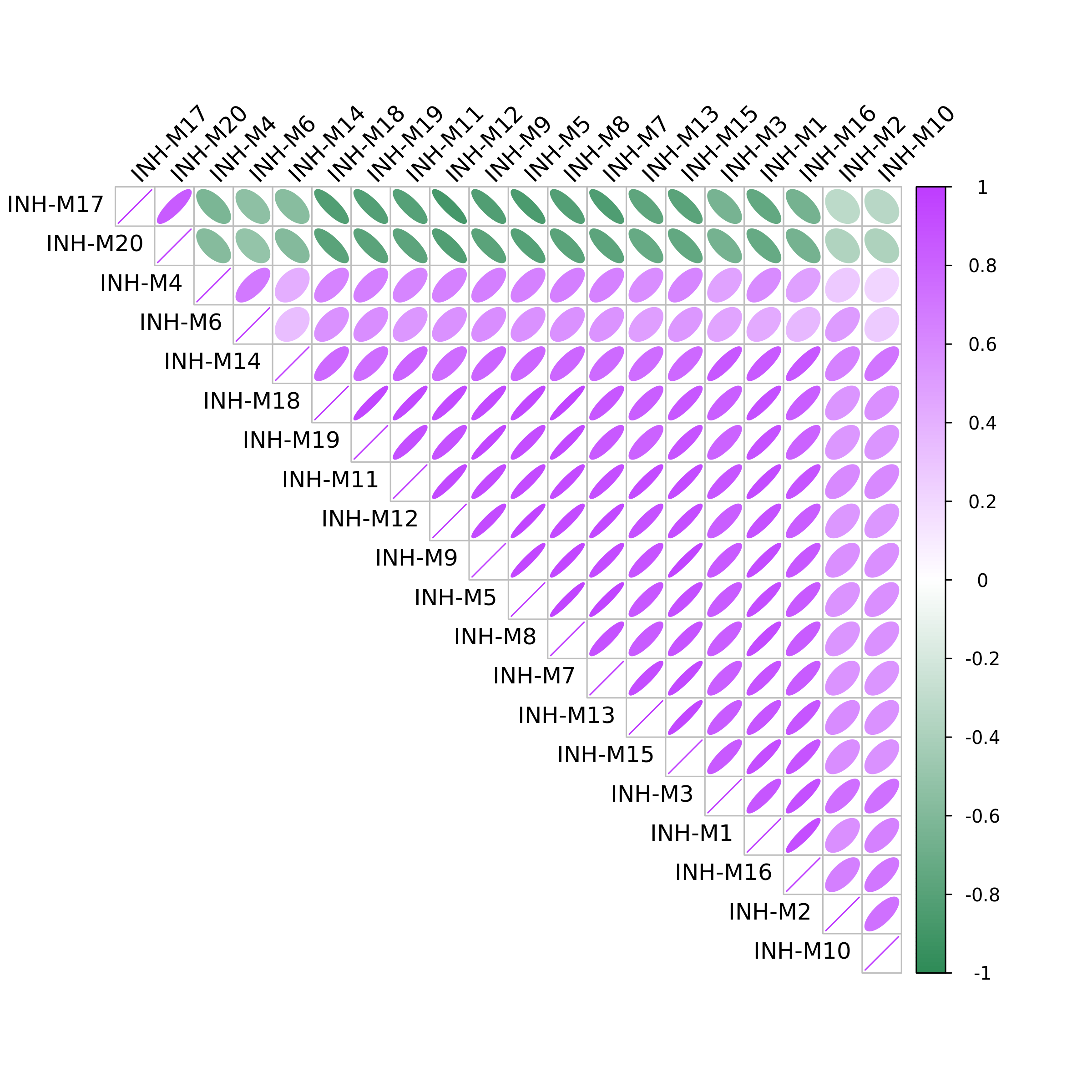
Plotting beyond the hdWGCNA package
Sometimes we want to make a custom visualization that may not be
included in hdWGCNA. Fortunately, R has an incredible amount of
different data visualization packages to take advantage of. The base
Seurat plotting functions are also great for visualizing hdWGCNA
outputs. Here is a simple example where we visualize the MEs using the
Seurat DotPlot function. The key to using Seurat’s plotting
functions to visualize the hdWGCNA data is to add it into the Seurat
object’s @meta.data slot.
# get hMEs from seurat object
MEs <- GetMEs(seurat_obj, harmonized=TRUE)
modules <- GetModules(seurat_obj)
mods <- levels(modules$module); mods <- mods[mods != 'grey']

# add hMEs to Seurat meta-data:
seurat_obj@meta.data <- cbind(seurat_obj@meta.data, MEs)
Now we can easily use Seurat’s DotPlot function:
# plot with Seurat's DotPlot function
p <- DotPlot(seurat_obj, features=mods, group.by = 'cell_type')

# flip the x/y axes, rotate the axis labels, and change color scheme:
p <- p +
  RotatedAxis() +
  scale_color_gradient2(high='red', mid='grey95', low='blue')

# plot output
p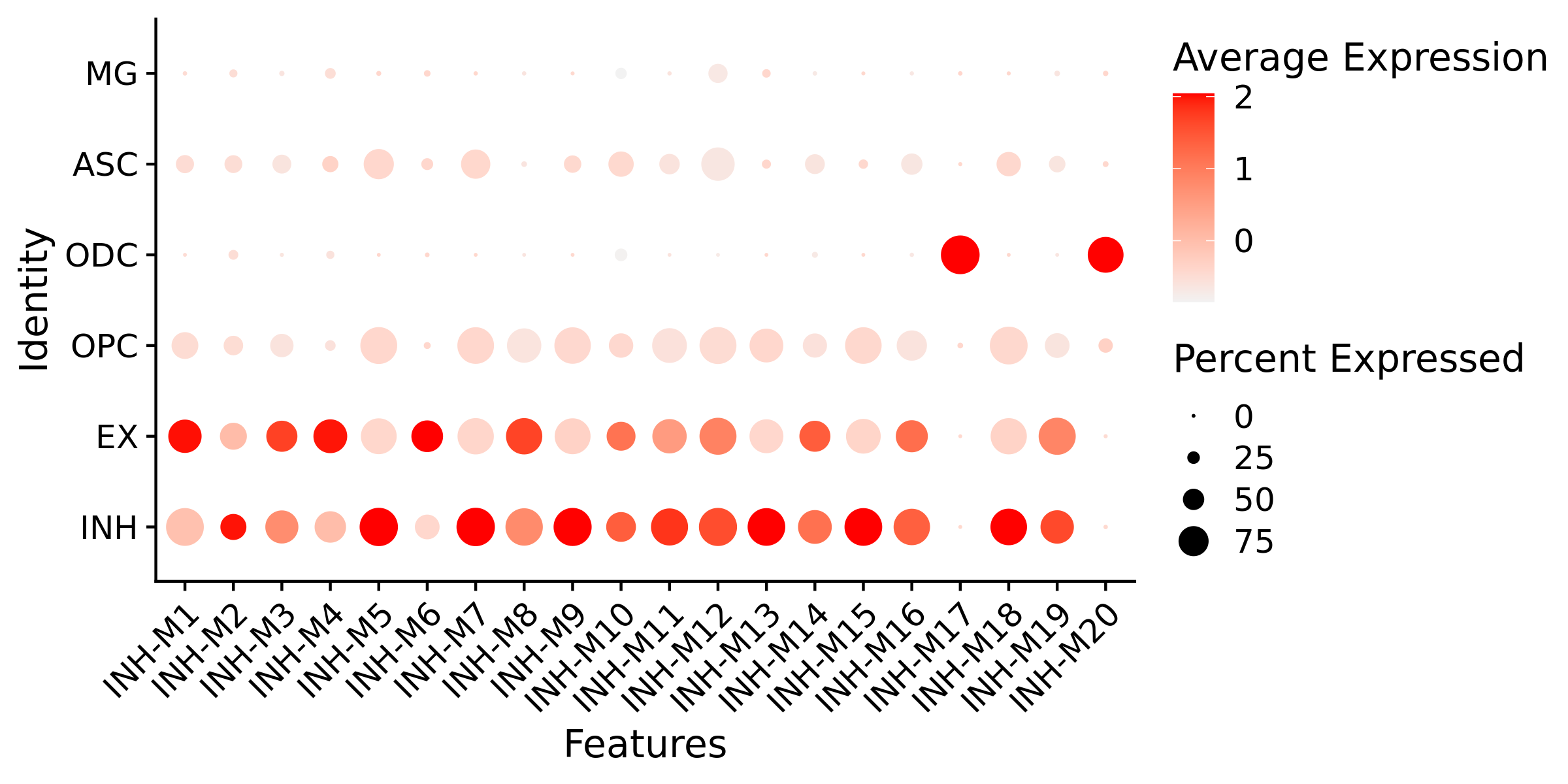
Next steps
Now that you have constructed a co-expression network and identified gene modules, there are many downstream analysis tasks which you can take advantage of within hdWGCNA. To provide more depth to your co-expression modules, we encourage you to explore the network visualization tutorial and the enrichment analysis tutorial.
To compare different biological conditions using hdWGCNA, check out the following tutorials.
- Differential module eigengene (DME) tutorial
- Module preservation tutorial
- Module-trait correlation tutorial
For more advanced analysis, such as Transcription factor regulatory network analysis, please check out the following tutorials.
- Transcription factor regulatory network analysis tutorial
- Protein-protein interaction tutorial
- Consensus network analysis tutorial
For those interested in running hdWGCNA using pseudobulk replicates rather than metacells, please check out this tutorial.