Module Trait Correlation • hdWGCNA

In this tutorial, we cover how to relate co-expression modules to biological and technical variables. Before starting this tutorial, make sure that you have constructed the co-expression network as in the hdWGCNA basics.

First Load the snRNA-seq data and the required libraries:

# single-cell analysis package
library(Seurat)

# plotting and data science packages
library(tidyverse)
library(cowplot)
library(patchwork)

# co-expression network analysis packages:
library(WGCNA)
library(hdWGCNA)

# using the cowplot theme for ggplot
theme_set(theme_cowplot())

# load the Zhou et al snRNA-seq dataset
seurat_ref <- readRDS('data/Zhou_control.rds')

Compute correlations

Here we use the function ModuleTraitCorrelation to correlate selected variables with module eigengenes. This function computes correlations for specified groupings of cells, since we can expect that some variables may be correlated with certain modules in certain cell groups but not in others. There are certain types of variables that can be used for this analysis while others should not be used.

Variables that can be used

Numeric variables
Categorical variables with only 2 categories, such as “control” and “condition”.
Categorical variables with a sequential relationship. For example, you may have a “disease stage” category ordered by “healthy”, “stage 1”, “stage 2”, “stage 3”, etc. In this case, you must ensure that the variable is stored as a factor and that the levels are set appropriately.

Variables that can not be used

Categorical variables with more than two categories that are not sequentially linked. For example, suppose you have a dataset consiting of three strains of transgenic mice and one control. Categorical variables must be converted to numeric before running the correlation, so you will end up with a correlation that is not at all biologically meaningful since there’s not a way to order the three different strains in a way that makes sense as a numeric variable. In this case, you should just set up a pairwise correlation between control and each strain separately. We often have a “Sample ID” variable indicating which cell came from which sample, and this is a variable that does not necessarily make sense to order in any particular way, so a variable like this would not be suitable for module-trait correlation analysis.

# convert sex to factor
seurat_obj$msex <- as.factor(seurat_obj$msex)

# convert age_death to numeric
seurat_obj$age_death <- as.numeric(seurat_obj$age_death)

# list of traits to correlate
cur_traits <- c('braaksc', 'pmi', 'msex', 'age_death', 'doublet_scores', 'nCount_RNA', 'nFeature_RNA', 'total_counts_mt')

seurat_obj <- ModuleTraitCorrelation(
  seurat_obj,
  traits = cur_traits,
  group.by='cell_type'
)

For any categorical variables used, this function prints out a warning message to tell the user what order the categories are listed in, just to make sure that it makes sense.

See warning message

Warning message:
In ModuleTraitCorrelation(seurat_obj, traits = cur_traits, group.by = "cell_type") :
  Trait msex is a factor with levels 0, 1. Levels will be converted to numeric IN THIS ORDER for the correlation, is this the expected order?

Inspecting the output

We can run the function GetModuleTraitCorrelation to retrieve the output of this function.

# get the mt-correlation results
mt_cor <- GetModuleTraitCorrelation(seurat_obj)

names(mt_cor)

[1] "cor"  "pval" "fdr"

mt_cor is a list containing three items; cor which holds the correlation results, pval which holds the correlation p-values, and fdr which holds the FDR-corrected p-values.

Each of these items is a list where each element is a dataframe for each of the correlation tests that were performed.

names(mt_cor$cor)

[1] "all_cells" "INH"       "EX"        "OPC"       "ODC"       "ASC"
[7] "MG"

 head(mt_cor$cor$INH[,1:5])

INH-M1       INH-M2       INH-M3      INH-M4        INH-M5
braaksc         0.040786737  0.090483529 -0.032898347  0.07570061 -0.0156434561
pmi             0.018372836 -0.030364143  0.035579410 -0.01642725  0.0004368311
msex           -0.032901606  0.009628401  0.014598909  0.00144740 -0.0126589860
age_death      -0.106830840 -0.154190736  0.000779827 -0.14647123  0.0080354876
doublet_scores  0.005359932  0.004313248 -0.282622533 -0.20010529 -0.2921721048
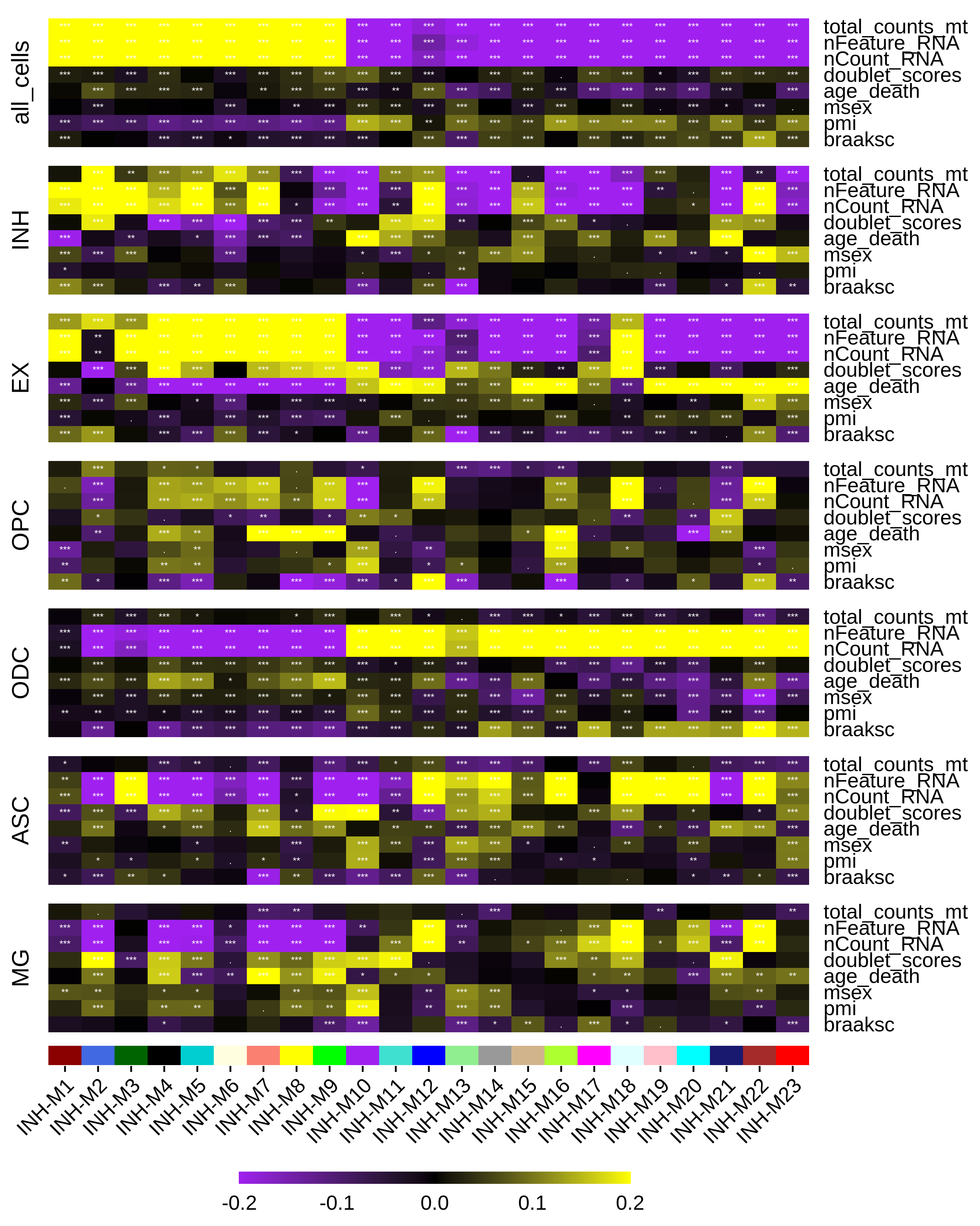
nCount_RNA     -0.192697871 -0.176522750 -0.427046078 -0.41516830 -0.1119312303

Plot Correlation Heatmap

We can plot the results of our correlation analysis using the PlotModuleTraitCorrelation function. This function creates a separate heatmap for each of the correlation matrices, and then assembles them into one plot using patchwork.

PlotModuleTraitCorrelation(
  seurat_obj,
  label = 'fdr',
  label_symbol = 'stars',
  text_size = 2,
  text_digits = 2,
  text_color = 'white',
  high_color = 'yellow',
  mid_color = 'black',
  low_color = 'purple',
  plot_max = 0.2,
  combine=TRUE
)