hdWGCNA with pseudobulk data

Compiled: 11-02-2026

Source: vignettes/pseudobulk.Rmd

In this tutorial, we demonstrate how to run hdWGCNA using pseudobulk data as an alternative to metacells or metaspots. Pseudobulking is particularly advantageous for very large datasets where metacell construction can be computationally prohibitive.

Considerations and motivation for pseudobulk hdWGCNA

“Pseudobulk” refers to aggregating gene expression profiles from all cells belonging to a specific group (e.g., cluster or cell type) within a single biological replicate. This process is analogous to physically sorting a cell population (e.g., via FACS) and performing bulk RNA-seq. While distinct from true bulk RNA-seq, this aggregation strategy effectively alleviates the sparsity of single-cell data, similar to our metacell approach.

A critical consideration for pseudobulk hdWGCNA is the number of biological replicates. Because single-cell and spatial experiments are costly, studies often feature a limited number of replicates.The original WGCNA FAQ page recommends a minimum of 20 samples to ensure that gene-gene correlations are robust and reproducible.

Load the dataset and required libraries

First we need to load the required libraries and the tutorial dataset into R.

library(Seurat)
library(tidyverse)
library(cowplot)
library(patchwork)
library(WGCNA)
library(hdWGCNA)
library(SummarizedExperiment)
theme_set(theme_cowplot())
set.seed(12345)
enableWGCNAThreads(nThreads = 8)

# load the Zhou et al snRNA-seq dataset
seurat_obj <- readRDS('Zhou_2020.rds')

Create the pseudobulk data matrix

Here we make the pseudobulk data matrix using the hdWGCNA function AggregatePseudobulk. This function sums the counts for all cells in a given group based on group_col in each biological replicate based on replicate_col, which should be metadata columns in seurat_obj@meta.data. This procedure returns a SummarizedExperiment object containing the pseudobulk dataset, with the corresponding meta-data automatically transferred from the Seurat object. We also normalize these pseudobulk counts using the NormalizeCounts function, which applies variance stabilizing transformation (VST) from the DESeq2 package by default.

seurat_obj <- SetupForWGCNA(
  seurat_obj,
  gene_select = "fraction", 
  fraction = 0.05, 
  wgcna_name = "pseudobulk"
)
length(GetWGCNAGenes(seurat_obj))

# get the counts matrix and the meta-data
X <- GetAssayData(seurat_obj, layer='counts')
meta <- seurat_obj@meta.data

# create a pseudo-bulk SummarizedExperiment object
se <- AggregatePseudobulk(
    X, meta, 
    replicate_col = "Sample", 
    group_col = "cell_type",
    assay_name = 'counts'
)

# normalize the pseudobulk SummarizedExperiment
se <- NormalizeCounts(
    se, 
    method = 'VST',
    assay_name = 'counts'
)

Co-expression network analysis

Now that we have our pseudobulk matrix, we can perform co-expression network analysis. First, we define the matrix that will be used for the analysis and we perform soft power thresholding.

# Set the pseudobulk matrix using the SummarizedExperiment object
seurat_obj <- SetDatExpr(
  seurat_obj,
  mat = se, layer = 'VST'
)

# select the soft power threshold
seurat_obj <- TestSoftPowers(seurat_obj)

We often want to subset to a specific group before constructing the co-expression network. This can easily be done by directly subsetting the SummarizedExperiment object and passing that to SetDatExpr.

# example only, not run for this tutorial.
seurat_obj <- SetDatExpr(
  seurat_obj,
  mat = se[,colData(se)$cell_type == 'ASC'], 
  layer = 'VST'
)

Now we are ready to construct the co-expression network and identify gene modules, which is done in the same way as with the metacell/metaspot data.

# construct the co-expression network and identify gene modules
seurat_obj <- ConstructNetwork(
    seurat_obj, 
    tom_name='pseudobulk', 
    overwrite_tom=TRUE,
    mergeCutHeight=0.15
)

PlotDendrogram(seurat_obj, main='pseudobulk dendrogram')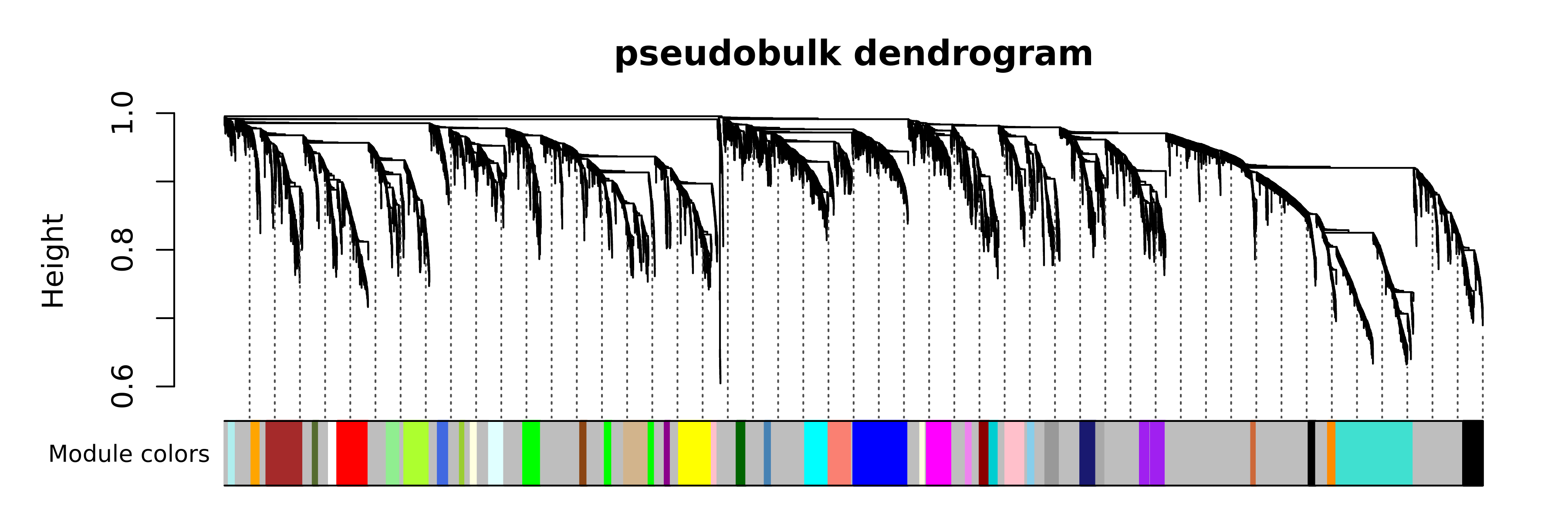

Next we compute the module eigengenes (MEs) and eigengene-based connectivity (kMEs) at the single-cell level, and we can plot the MEs for each module in the different cell types.

# compute the MEs and kMEs
seurat_obj <- ModuleEigengenes(seurat_obj)
seurat_obj <- ModuleConnectivity(seurat_obj)

# get MEs from seurat object
MEs <- GetMEs(seurat_obj)
mods <- colnames(MEs); mods <- mods[mods != 'grey']

# add MEs to Seurat meta-data for plotting:
meta <- seurat_obj@meta.data
seurat_obj@meta.data <- cbind(meta, MEs)

# plot with Seurat's DotPlot function
p <- DotPlot(seurat_obj, features=mods, group.by = 'cell_type')

# reset the metadata
seurat_obj@meta.data <- meta

# flip the x/y axes, rotate the axis labels, and change color scheme:
p <- p +
  RotatedAxis() +
  scale_color_gradient(high='red', low='grey95') + 
  xlab('') + ylab('')

p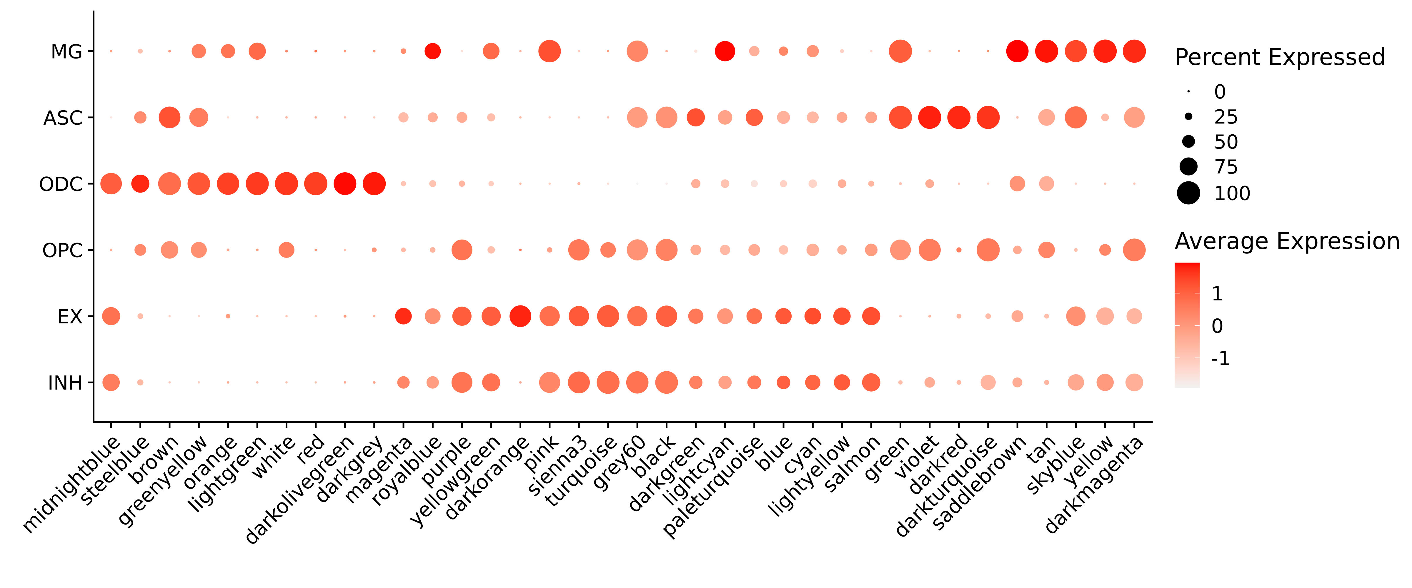 

Next we will use UMAP to project the co-expression network in two dimensions, and we will visualize the results using ggplot2.

# compute the co-expression network umap 
seurat_obj <- RunModuleUMAP(
  seurat_obj,
  n_hubs = 5,
  n_neighbors=10,
  min_dist=0.4,
  spread=3,
  supervised=TRUE,
  target_weight=0.3
)

# get the hub gene UMAP table from the seurat object
umap_df <- GetModuleUMAP(seurat_obj)

# plot with ggplot
p <- ggplot(umap_df, aes(x=UMAP1, y=UMAP2)) +
  geom_point(
   color=umap_df$color,
   size=umap_df$kME*2
  ) + 
  umap_theme() 

# add the module names to the plot by taking the mean coordinates
centroid_df <- umap_df %>% 
  dplyr::group_by(module) %>%
  dplyr::summarise(UMAP1 = mean(UMAP1), UMAP2 = mean(UMAP2))
 
p <- p + geom_label(
  data = centroid_df, 
  label=as.character(centroid_df$module), 
  fontface='bold', size=2) + 
  theme(panel.background = element_rect(fill='black'))

p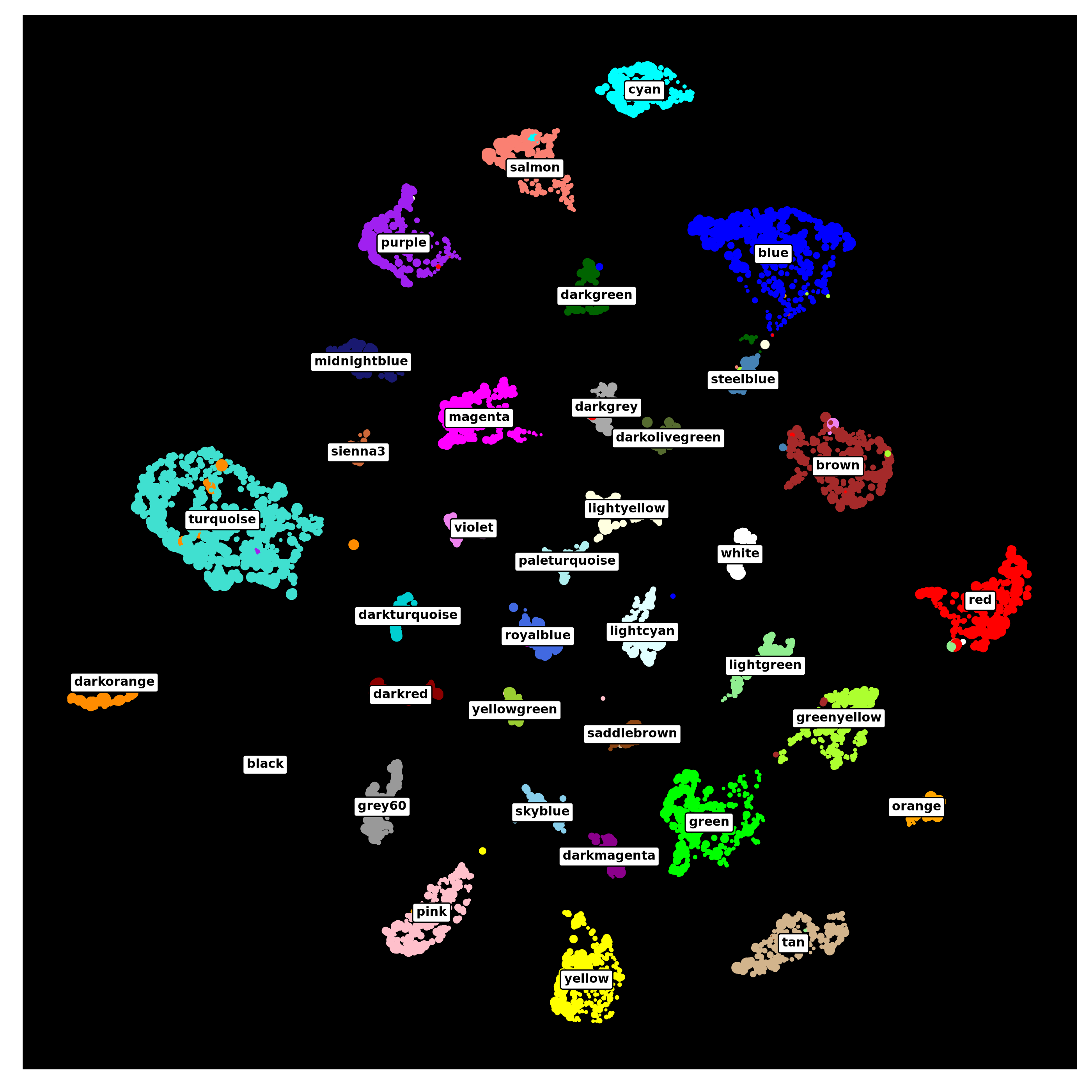

As you can see, the co-expression network derived from pseudobulk data can be used for the same downstream analysis as with the metacell/metaspot data.

Consensus network analysis with pseudobulk data

We can also run consensus network analysis using pseudobulk data. If you are not already familiar
with consensus co-expression network analysis, please visit our other tutorial page describing it in more detail. Here we will use all cell types again, and we will run the consensus network analysis with biological sex as the variable of interest. When we run ConstructPseudobulk, we have to provide the function with information about the cell groupings, the biological samples, and the variable we will be using for consensus network analysis (sex in this case).

# set up a new wgcna experiment for the consensus analysis
seurat_obj <- SetupForWGCNA(
  seurat_obj,
  gene_select = "fraction",
  fraction = 0.05,
  wgcna_name = "pseudobulk_consensus"
)

# casting sex to a factor or else it will give an error!!
seurat_obj$msex <- as.factor(seurat_obj$msex)

# get the counts matrix and the meta-data
X <- GetAssayData(seurat_obj, layer='counts')
meta <- seurat_obj@meta.data

# create a pseudo-bulk SummarizedExperiment object (same as before)
se <- AggregatePseudobulk(
    X, meta, 
    replicate_col = "Sample", 
    group_col = "cell_type",
    assay_name = 'counts'
)

# normalize the pseudobulk SummarizedExperiment (same as before)
se <- NormalizeCounts(
    se, 
    method = 'VST',
    assay_name = 'counts'
)

# set the multiExpr slot using the SummarizedExperiment object
seurat_obj <- SetMultiExpr(
  seurat_obj,
  layer = 'VST',
  multi.group.by='msex',
  mat = se
)

seurat_obj <- TestSoftPowersConsensus(seurat_obj)

# generate plots
plot_list <-  PlotSoftPowers(seurat_obj)

# get just the scale-free topology fit plot for each group
consensus_groups <- unique(seurat_obj$msex)
p_list <- lapply(1:length(consensus_groups), function(i){
  cur_group <- consensus_groups[[i]]
  plot_list[[i]][[1]] + ggtitle(paste0('Sex: ', cur_group)) + theme(plot.title=element_text(hjust=0.5))
})

wrap_plots(p_list, ncol=2)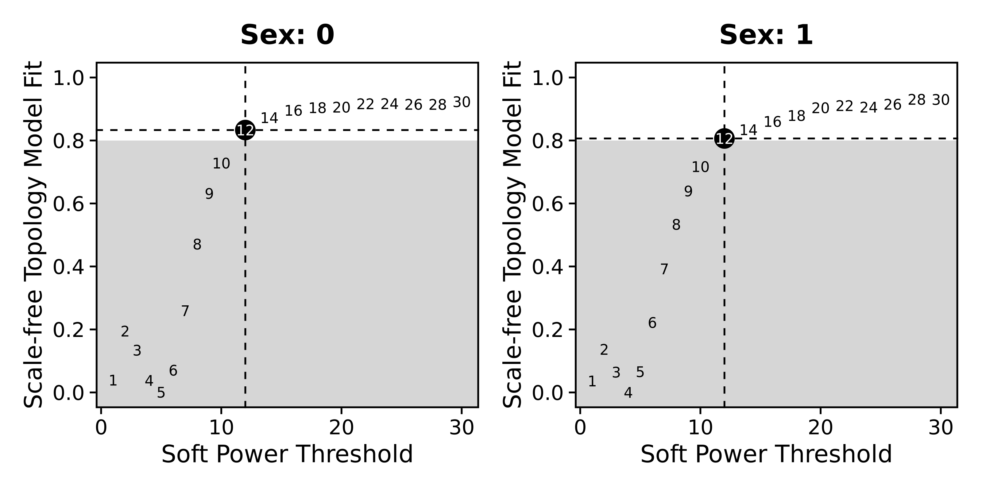

We now proceed with the network construction, and we ensure to set consensus=TRUE.

seurat_obj <- ConstructNetwork(
  seurat_obj,
  consensus=TRUE,
  tom_name = "pseudobulk_consensus",
  overwrite_tom=TRUE,
  mergeCutHeight=0.1
)

# plot the dendrogram
PlotDendrogram(seurat_obj, main='pseudobulk consensus dendrogram')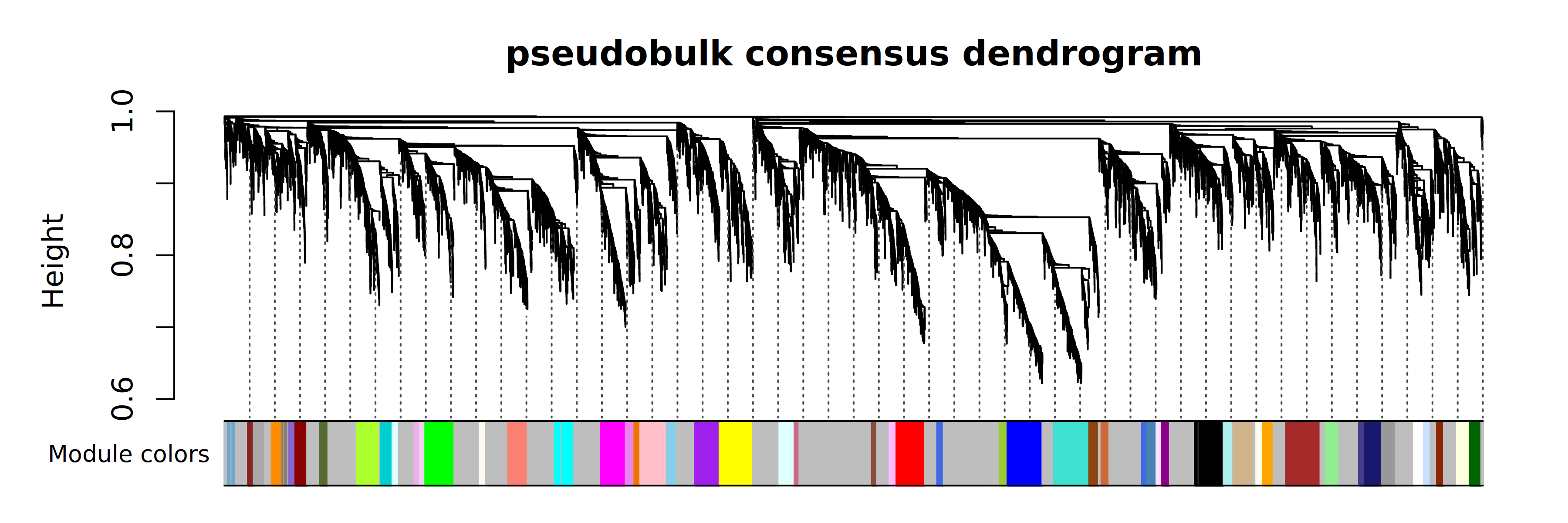

Finally we will compute the MEs and kMEs, and visualize the expression level of each of the 54 modules in the 6 major cell types.

# compute the MEs and kMEs
seurat_obj <- ModuleEigengenes(seurat_obj)
seurat_obj <- ModuleConnectivity(seurat_obj)

# get MEs from seurat object
MEs <- GetMEs(seurat_obj)
mods <- colnames(MEs); mods <- mods[mods != 'grey']

# add MEs to Seurat meta-data for plotting:
meta <- seurat_obj@meta.data
seurat_obj@meta.data <- cbind(meta, MEs)

# plot with Seurat's DotPlot function
p <- DotPlot(seurat_obj, features=mods, group.by = 'cell_type')

# reset the metadata to remove the MEs
seurat_obj@meta.data <- meta

# flip the x/y axes, rotate the axis labels, and change color scheme:
p <- p +
  RotatedAxis() +
  scale_color_gradient(high='red', low='grey95') + 
  xlab('') + ylab('')

p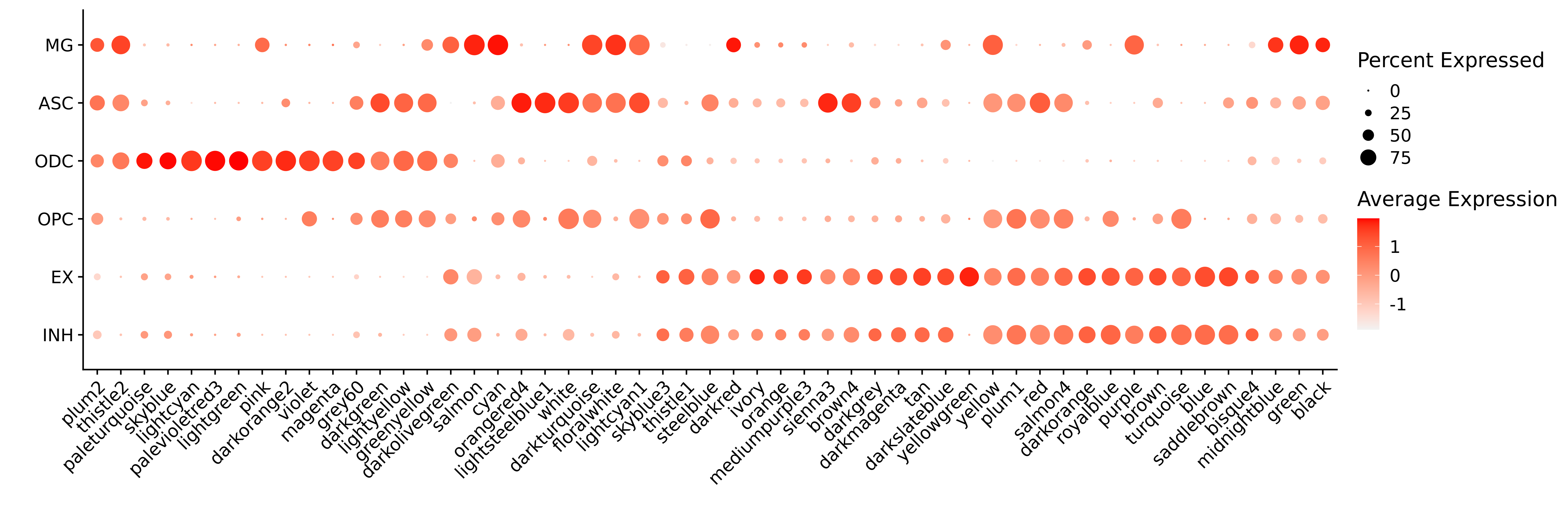

The tutorial ends here but the pseudobulk consensus modules can be further explored using our other tutorials.