Module preservation and reproducibility
Source:vignettes/module_preservation.Rmd
module_preservation.RmdCompiled: 28-05-2024
Source: vignettes/module_preservation.Rmd
Data-driven models are most useful when they are generalizable across different datasets. Thinking about co-expression networks from this perspective, we need a way to quantify and test the conservation of co-expression patterns identified in one dataset across external datasets. In this tutorial, we demonstrate module preservation analysis with hdWGCNA, a statistical framework that allows us to test the degree to which co-expression modules identified in one dataset are “preserved” in another dataset. Module preservation analysis can also be used to assess biological relevance of co-expression modules. For example, you can imagine that you may find modules in a disease samples that are not preserved in healthy samples, or you may find modules in humans that are not preserved in mice. This tutorial builds off of a previous tutorial, where we projected the co-expression modules from a reference dataset to a query dataset.
First we must load the data and the required libraries:
# single-cell analysis package
library(Seurat)

# plotting and data science packages
library(tidyverse)
library(cowplot)
library(patchwork)

# co-expression network analysis packages:
library(WGCNA)
library(hdWGCNA)

# network analysis & visualization package:
library(igraph)

# using the cowplot theme for ggplot
theme_set(theme_cowplot())

# set random seed for reproducibility
set.seed(12345)

# load the Zhou et al snRNA-seq dataset
seurat_ref <- readRDS('data/Zhou_control.rds')

# load the Morabito & Miyoshi 2021 snRNA-seq dataset
seurat_query <- readRDS(file=paste0(data_dir, 'Morabito_Miyoshi_2021_control.rds'))
Module preservation analysis
In their 2011 paper titled “Is My Network Module Preserved and Reproducible?”, Langfelder et al discuss statistical methods for module preservation analysis in co-expression network analysis. Notably, module preservation analysis can be used to assess the reproducibility of co-expression networks, but it can also be used for specific biological analyses, for example to identify which modules are significantly preserved across different disease conditions, tissues, developmental stages, or even evolutionary time.
The first step in module preservation analysis is to project modules from a reference to a query dataset, which is explained in more detail in the previous tutorial.
seurat_query <- ProjectModules(
  seurat_obj = seurat_query,
  seurat_ref = seurat_ref,
  wgcna_name = "tutorial",
  wgcna_name_proj="projected",
  assay="RNA" # assay for query dataset
)
Next, we set up the expression matrices for the query and reference
datasets. Either the single-cell or the metacell gene expression
matrices can be used here by setting the use_metacells flag
in SetDatExpr. In general we recommend using the same
matrix that was used to construct the network for the reference (in this
case, the metacell matrix). If you have not already constructed
metacells in the query dataset, you can do that prior to module
preservation analysis.
See code to consruct metacells in the query dataset
# construct metacells:
seurat_query <- MetacellsByGroups(
  seurat_obj = seurat_query,
  group.by = c("cell_type", "Sample"),
  k = 25,
  max_shared = 12,
  reduction = 'harmony',
  ident.group = 'cell_type'
)
seurat_query <- NormalizeMetacells(seurat_query)
# set expression matrix for reference dataset
seurat_ref <- SetDatExpr(
  seurat_ref,
  group_name = "INH",
  group.by = "cell_type"
)

# set expression matrix for query dataset:
seurat_query <- SetDatExpr(
  seurat_query,
  group_name = "INH",
  group.by = "cell_type"
)
Now we can run the ModulePreservation function. Note
that this function does take a while to run since it is a permutation
test, but it can be sped up by lowering the n_permutations
parameter, but we do not recommend any lower than 100 permutations. Also
note that the parallel option currently does not work. For
demonstration purposes, we ran the code for this tutorial using only 20
permutations so it would run quickly.
ModulePreservation takes a name parameter,
which is used to store the results of this module perturbation test.
# run module preservation function
seurat_query <- ModulePreservation(
  seurat_query,
  seurat_ref = seurat_ref,
  name="Zhou-INH",
  verbose=3,
  n_permutations=250 # n_permutations=20 used for the tutorial
)
Visualize preservation stats
The module perturbation test produces a number of different preservation statistics, which you can inspect in the following tables.
# get the module preservation table
mod_pres <- GetModulePreservation(seurat_query, "Zhou-INH")$Z
obs_df <- GetModulePreservation(seurat_query, "Zhou-INH")$obs
In the past we linked to the original WGCNA documentation website for more detailed explanations of thes statistics, but unfortunately at the time of writing this tutorial the website has been taken offline. Please refer to the original publication in PLOS Computational Biology for further explanations.
hdWGCNA includes the function PlotModulePreservation to
visualize the statistics we computed in the previous section. This
function generates a scatter plot showing the module size versus the
module preservation stats. The summary statistics aggregate the
individual preservation and quality statistics into a single metric so
we generally recommend primarily interpreting the results with these
plots.
plot_list <- PlotModulePreservation(
  seurat_query,
  name="Zhou-INH",
  statistics = "summary"
)

wrap_plots(plot_list, ncol=2)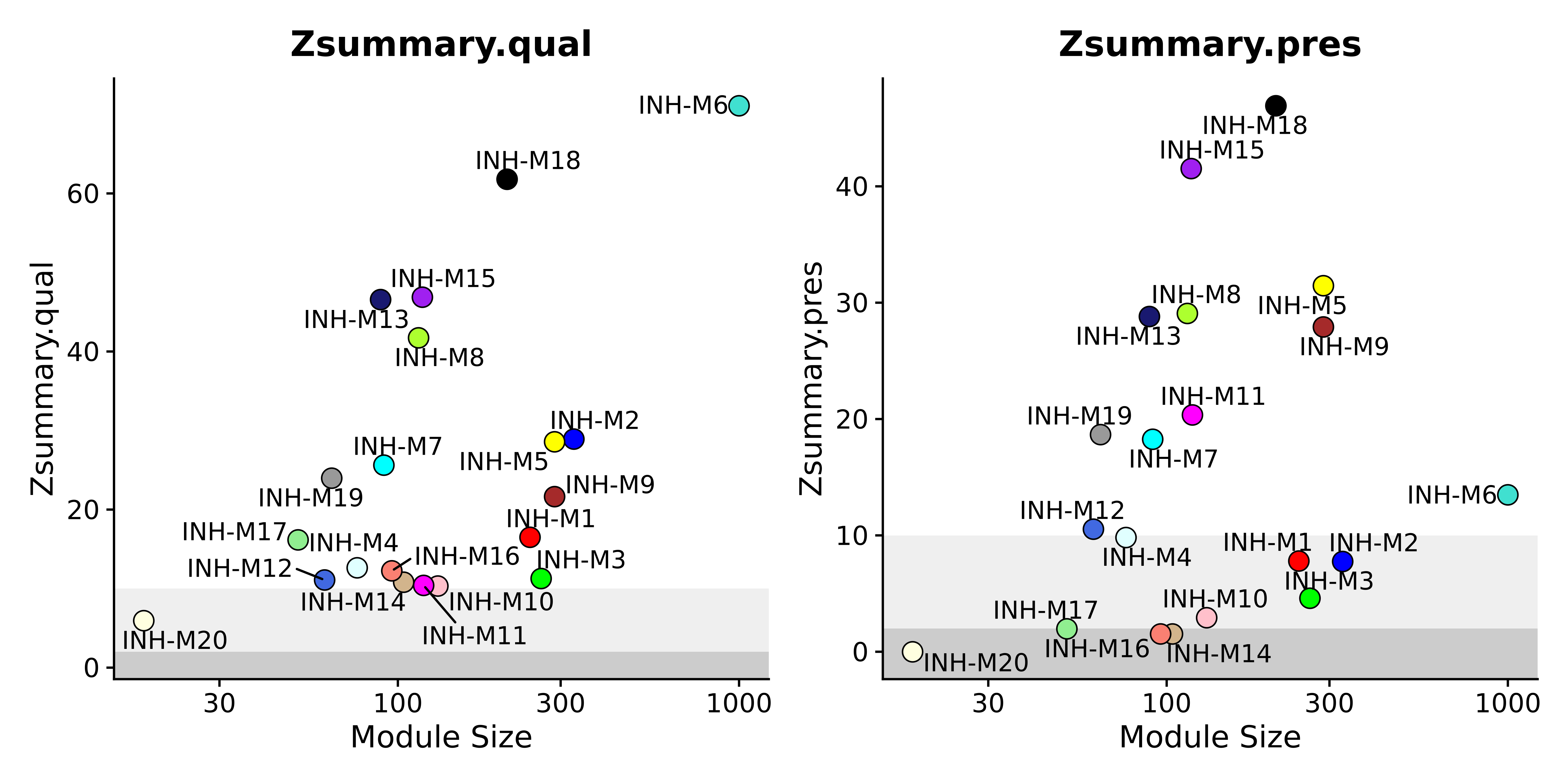
Here we can see three different shades in the background. These represent cutoff values for interpreting the Z summary statistics. The following guidelines help us understand the preservation of these modules.
- Z < 2, the module is not preserved in the query dataset.
- 10 > Z > 2, the module is moderately preserved in the query dataset.
- Z > 10, the module is highly preserved in the query dataset.
The following code shows how to plot additional module preservation stats.
# plot ranking stats
plot_list <- PlotModulePreservation(
  seurat_query,
  name="Zhou-INH",
  statistics = "rank"
)


wrap_plots(plot_list, ncol=2)![]()
Plot all of the different stats:
plot_list <- PlotModulePreservation(
  seurat_query,
  name="Zhou-INH",
  statistics = "all",
  plot_labels=FALSE
)

wrap_plots(plot_list, ncol=6)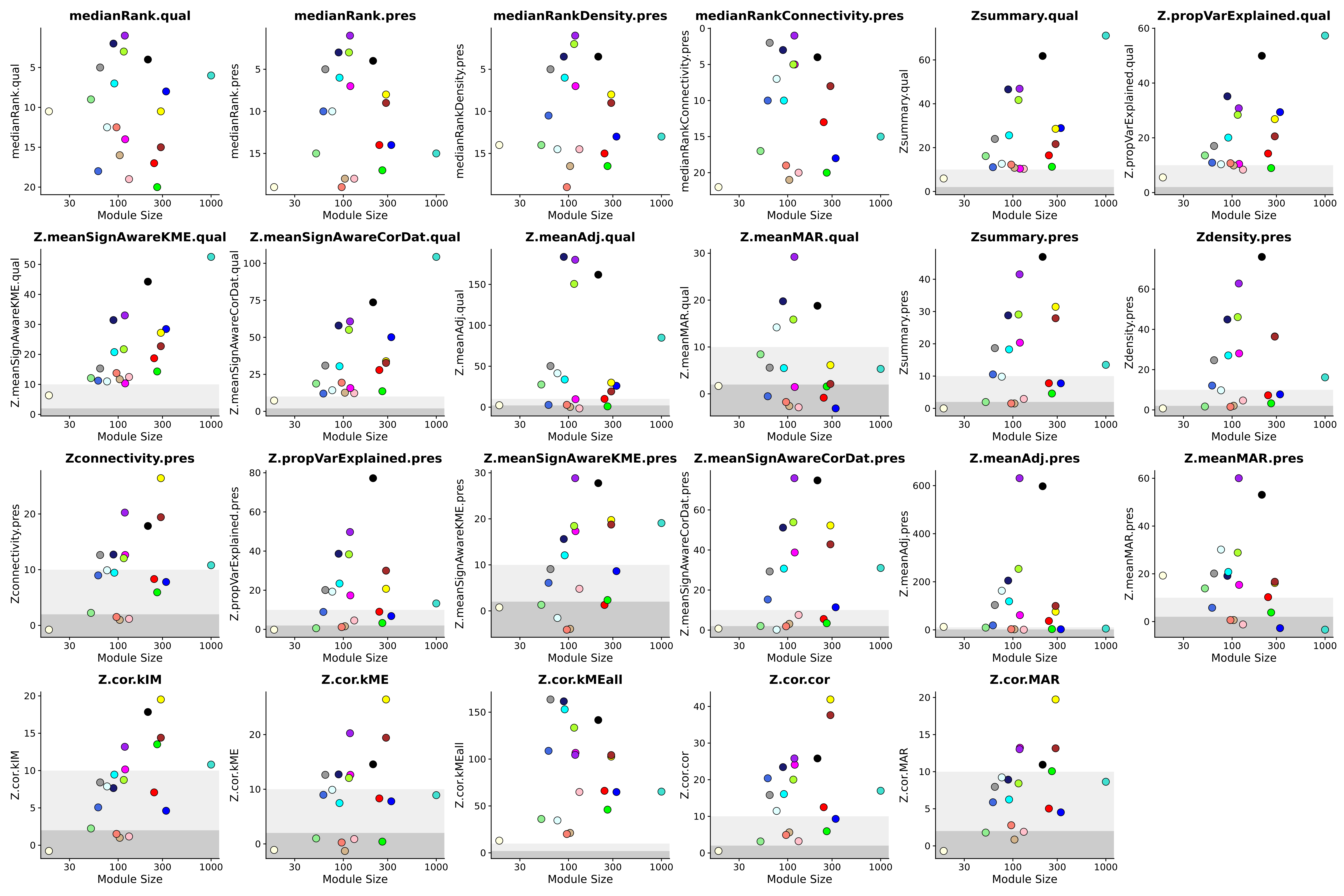
Module preservation analysis with NetRep
Here we include an alternative method for performing module
preservation analysis using the R package NetRep. In
their 2016 paper titled “A Scalable
Permutation Approach Reveals Replication and Preservation Patterns of
Network Modules in Large Datasets”, Ritchie et al. introduced a
relatively faster approach for module preservation. In this paper, the
authors also show that this method has improved false discovery control.
We include a function ModulePreservationNetRep in order to
perform this analysis in hdWGCNA. NetRep is not included as
a dependency of hdWGCNA since it is not used for other analyses, so here
we must install NetRep before proceeding.
If you use this method in your research, we encourage you to properly
cite the NetRep paper. Please consult the NetRep GitHub
repository for more details.
# install
install.packages('NetRep')
One important difference between these two implementations of module preservation analysis is that NetRep requires the topological overlap matrix (TOM) for the query and for the reference datasets. In order to satisfy this requirement, we first perform the standard hdWGCNA analysis on the query dataset.
See code to perform network analysis in the query dataset
# use the genes from the ref dataset
genes_use <- GetWGCNAGenes(seurat_ref)
seurat_query <- SetupForWGCNA(
  seurat_query,
  features = genes_use,
  wgcna_name = "INH"
)

# construct metacells:
seurat_query <- MetacellsByGroups(
  seurat_obj = seurat_query,
  group.by = c("cell_type", "Sample"),
  k = 25,
  max_shared = 12,
  reduction = 'harmony',
  ident.group = 'cell_type'
)
seurat_query <- NormalizeMetacells(seurat_query)


seurat_query <- SetDatExpr(
  seurat_query,
  group_name = "INH",
  group.by='cell_type'
)

# Test different soft powers:
seurat_query <- TestSoftPowers(
  seurat_query,
  networkType = 'signed'
)

# construct co-expression network:
seurat_query <- ConstructNetwork(
  seurat_query,
  tom_name = 'INH_query',
  overwrite_tom=TRUE
)

# compute all MEs in the full single-cell dataset
seurat_query <- ModuleEigengenes(seurat_query)

# compute eigengene-based connectivity (kME):
seurat_query <- hdWGCNA::ModuleConnectivity(
  seurat_query,
  group.by = 'cell_type', group_name = 'INH'
)

# reset the active WGCNA to projected
seurat_query <- SetActiveWGCNA(seurat_query, 'projected')
Next we can run the ModulePreservationNetRep function to
perform module preservation analysis using the NetRep
method.
# run NetRep module preservation
seurat_query <- ModulePreservationNetRep(
  seurat_query,
  seurat_ref,
  name = 'testing_NetRep',
  n_permutations = 5000,
  n_threads=8, # number of threads to run in Parallel
  TOM_use="INH", # specify the name of the hdWGCNA experiment that contains the TOM for the query dataset
  wgcna_name = 'projected',
  wgcna_name_ref = 'tutorial'
)

# access the results:
mod_pres <- GetModulePreservation(seurat_query, 'testing_NetRep', 'projected')

# access statistics for each module:
mod_pres$p.values
This approach reports preservation statistics for each module, and in
this case a significant p-value indicates that a given module is
significantly preserved. NetRep reports p-values for seven
different network attributes, so we can see specifically which
attributes are preserved or not. To get an overall result of module
preservation, we compute the average of these different p-values.
Next we plot the resulting statistics using the function
PlotModulePreservationLollipop.
PlotModulePreservationLollipop(
  seurat_query,
  name='testing_NetRep',
  features='average',
  wgcna_name='projected'
) + RotatedAxis() + NoLegend()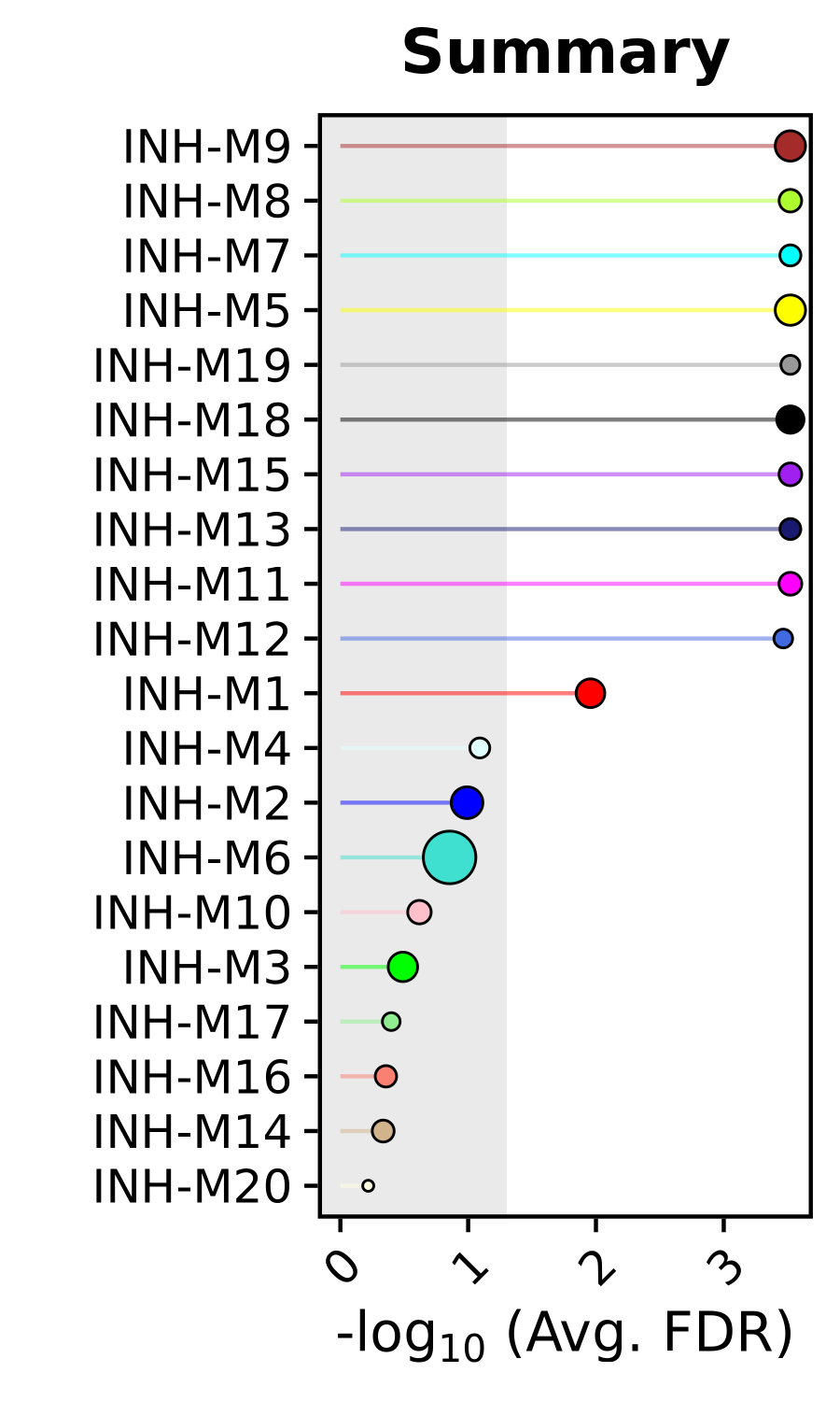
This plot shows us each module ranked by how well they module
preserved in the query dataset. The x-axis is showing us the averaged
FDR-corrected p-values from the different network attributes for each
module to result in a composite statistic. The size of each dot
corresponds to the number of genes in each module. We can also use this
same function to plot the individual statistics. As a demonstration we
also set fdr=FALSE to show how to look at the raw p-value
rather than the FDR-corrected p-value based on the user’s
preference.
# get the module preservation results
mod_pres <- GetModulePreservation(seurat_query, 'testing_NetRep', 'projected')

# get the names of the statistics to plot
plot_features <- c('average', colnames(mod_pres$p.value))

# loop through each statistic
plot_list <- list()
for(cur_feature in plot_features){
    plot_list[[cur_feature]] <- PlotModulePreservationLollipop(
    seurat_query,
    name='testing_NetRep',
    features=cur_feature,
    fdr=FALSE,
    wgcna_name='projected'
  ) + RotatedAxis() + NoLegend()
}

# assemble the final plot
wrap_plots(plot_list, ncol=4)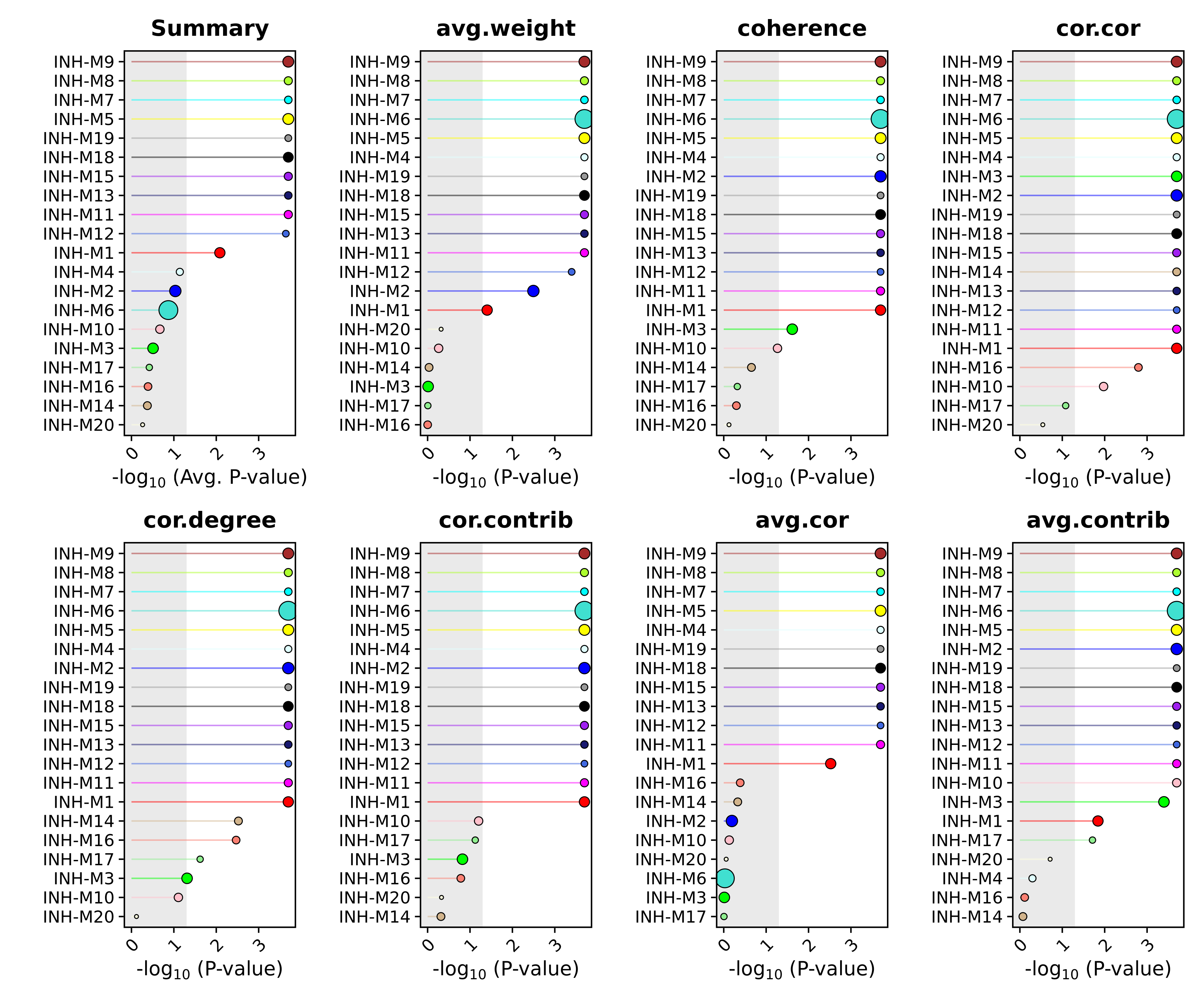
Module topology comparisons
Here we demonstrate several functions to help visually compare the
network topology of a co-expression module in two different datasets.
This can be useful to visualize some modules of interest based on the
results of the module preservation test. The function
ModuleTopologyHeatmap generates a heatmap showing the
gene-gene co-expression matrix, either colored by the correlation value
or the edge weight in the TOM. In this plot, genes are sorted by their
intramodular connectivity. Additionally,
ModuleTopologyBarplot complements this by showing the
connectivity of each gene (network degree or kME value) in each
module.
In order to compare the module topology between a reference and a
query dataset, we require a co-expression network (TOM) for both
datasets. The TOM is only calculated by the
ConstructNetwork function, not ProjectModules,
so we first need to run this step on the query dataset.
# get the list of genes in the reference object
genes_use <- GetWGCNAGenes(seurat_ref)

seurat_query <- SetupForWGCNA(
  seurat_query,
  features = genes_use,
  wgcna_name = "INH",
)

# construct metacells:
seurat_query <- MetacellsByGroups(
  seurat_obj = seurat_query,
  group.by = c("cell_type", "Sample"),
  k = 25,
  max_shared = 12,
  reduction = 'harmony',
  ident.group = 'cell_type'
)
seurat_query <- NormalizeMetacells(seurat_query)

seurat_query <- SetDatExpr(
  seurat_query,
  group_name = "INH",
  group.by='cell_type',
  assay = 'RNA',
  layer = 'data'
)

seurat_query <- TestSoftPowers(seurat_query)
seurat_query <- ConstructNetwork(seurat_query, tom_name = 'INH_query')
seurat_query <- ModuleEigengenes(seurat_query)
seurat_query <- ModuleConnectivity(
  seurat_query,
  group.by = 'cell_type', group_name = 'INH'
)

# reset the active WGCNA to the projected
seurat_query <- SetActiveWGCNA(seurat_query, 'projected')
We will make a patchwork plot showing the correlation heatmap, the TOM heatmap, the degree barplot, and the kME barplot for module INH-M9, which showed significant preservation based on both module preservation approaches. To better visually compare these plots side-by-side, we must ensure that the genes are ordered the same way. Here we will order the genes based on the reference dataset.
# select the module to plot
cur_mod <- 'INH-M9'

# plot the correlation matrix in the reference dataset
tmp <- ModuleTopologyHeatmap(
    seurat_ref,
    mod = cur_mod,
    matrix = "Cor",
    order_by = 'degree',
    TOM_use = 'tutorial',
    wgcna_name = 'tutorial',
    high_color = 'red',
    type = 'unsigned',
    plot_max = 0.75,
    return_genes = TRUE # select this option to get the gene order
)

# get the plot from the output list
p1 <- tmp[[1]] + ggtitle('Reference') + ylab('Correlation') + NoLegend()

# get the gene order from the output list
gene_list <- tmp[[2]]

# plot the correlation matrix in the query dataset
p2 <- ModuleTopologyHeatmap(
    seurat_query,
    mod = cur_mod,
    matrix = "Cor",
    order_by = 'degree',
    wgcna_name = 'projected',
    high_color = 'red',
    type = 'unsigned',
    plot_max = 0.75,
    genes_order = gene_list
) + ggtitle('Query')

# plot the TOM in the reference dataset
p3 <- ModuleTopologyHeatmap(
    seurat_ref,
    mod = cur_mod,
    matrix = "TOM",
    order_by = 'degree',
    wgcna_name = 'tutorial',
    high_color = 'seagreen',
    genes_order = gene_list,
    plot_max = 0.05
) + ylab('Network edge weight') + NoLegend()

# plot the TOM in the query dataset
p4 <- ModuleTopologyHeatmap(
    seurat_query,
    mod = cur_mod,
    matrix = "TOM",
    order_by = 'degree',
    TOM_use = 'INH',
    wgcna_name = 'projected',
    high_color = 'seagreen',
    plot_max = 0.05,
    genes_order = gene_list
)


# plot the degree in the reference dataset
p5 <- ModuleTopologyBarplot(
    seurat_ref,
    mod = cur_mod,
    features = 'weighted_degree',
    genes_order = gene_list,
    wgcna_name = 'tutorial',
) + NoLegend()

# plot the degree in the query dataset
p6 <- ModuleTopologyBarplot(
    seurat_query,
    mod = cur_mod,
    features = 'weighted_degree',
    genes_order = gene_list,
    wgcna_name = 'projected'
)+ NoLegend()

# plot the kME in the reference dataset
tmp <- ModuleTopologyBarplot(
    seurat_ref,
    mod = cur_mod,
    features = 'kME',
    wgcna_name = 'tutorial',
    return_genes=TRUE
)
p7 <- tmp[[1]] + NoLegend()
gene_list2 <- tmp[[2]]

# plot the kME in the query dataset
p8 <- ModuleTopologyBarplot(
    seurat_query,
    mod = cur_mod,
    features = 'kME',
    genes_order = gene_list2,
    wgcna_name = 'projected'
)+ NoLegend()

# assemble patch:
patch <- (p1 | p2) / (p3 | p4) / (p5 | p6) / (p7 | p8) +
    plot_layout(heights=c(3,3,1,1)) &
    plot_annotation(title = paste0(cur_mod, ' topology comparison')) &
    theme(plot.title=element_text(hjust=0.5))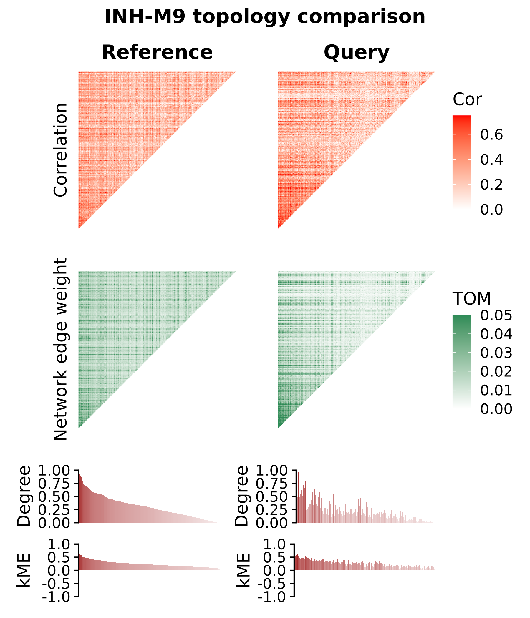
As another example, we can create a similar plot for a module which was not significantly preserved in the query dataset, INH-M2.
See code to plot network topology for INH-M2
# select the module to plot
cur_mod <- 'INH-M2'

# plot the correlation matrix in the reference dataset
tmp <- ModuleTopologyHeatmap(
    seurat_ref,
    mod = cur_mod,
    matrix = "Cor",
    order_by = 'degree',
    TOM_use = 'tutorial',
    wgcna_name = 'tutorial',
    high_color = 'red',
    type = 'unsigned',
    plot_max = 0.75,
    return_genes = TRUE # select this option to get the gene order
)

# get the plot from the output list
p1 <- tmp[[1]] + ggtitle('Reference') + ylab('Correlation') + NoLegend()

# get the gene order from the output list
gene_list <- tmp[[2]]

# plot the correlation matrix in the query dataset
p2 <- ModuleTopologyHeatmap(
    seurat_query,
    mod = cur_mod,
    matrix = "Cor",
    order_by = 'degree',
    wgcna_name = 'projected',
    high_color = 'red',
    type = 'unsigned',
    plot_max = 0.75,
    genes_order = gene_list
) + ggtitle('Query')

# plot the TOM in the reference dataset
p3 <- ModuleTopologyHeatmap(
    seurat_ref,
    mod = cur_mod,
    matrix = "TOM",
    order_by = 'degree',
    wgcna_name = 'tutorial',
    high_color = 'seagreen',
    genes_order = gene_list,
    plot_max = 0.05
) + ylab('Network edge weight') + NoLegend()

# plot the TOM in the query dataset
p4 <- ModuleTopologyHeatmap(
    seurat_query,
    mod = cur_mod,
    matrix = "TOM",
    order_by = 'degree',
    TOM_use = 'INH',
    wgcna_name = 'projected',
    high_color = 'seagreen',
    plot_max = 0.05,
    genes_order = gene_list
)


# plot the degree in the reference dataset
p5 <- ModuleTopologyBarplot(
    seurat_ref,
    mod = cur_mod,
    features = 'weighted_degree',
    genes_order = gene_list,
    wgcna_name = 'tutorial',
) + NoLegend()

# plot the degree in the query dataset
p6 <- ModuleTopologyBarplot(
    seurat_query,
    mod = cur_mod,
    features = 'weighted_degree',
    genes_order = gene_list,
    wgcna_name = 'projected'
)+ NoLegend()

# plot the kME in the reference dataset
tmp <- ModuleTopologyBarplot(
    seurat_ref,
    mod = cur_mod,
    features = 'kME',
    wgcna_name = 'tutorial',
    return_genes=TRUE
)
p7 <- tmp[[1]] + NoLegend()
gene_list2 <- tmp[[2]]

# plot the kME in the query dataset
p8 <- ModuleTopologyBarplot(
    seurat_query,
    mod = cur_mod,
    features = 'kME',
    genes_order = gene_list2,
    wgcna_name = 'projected'
)+ NoLegend()

# assemble patch:
patch <- (p1 | p2) / (p3 | p4) / (p5 | p6) / (p7 | p8) +
    plot_layout(heights=c(3,3,1,1)) &
    plot_annotation(title = paste0(cur_mod, ' topology comparison')) &
    theme(plot.title=element_text(hjust=0.5))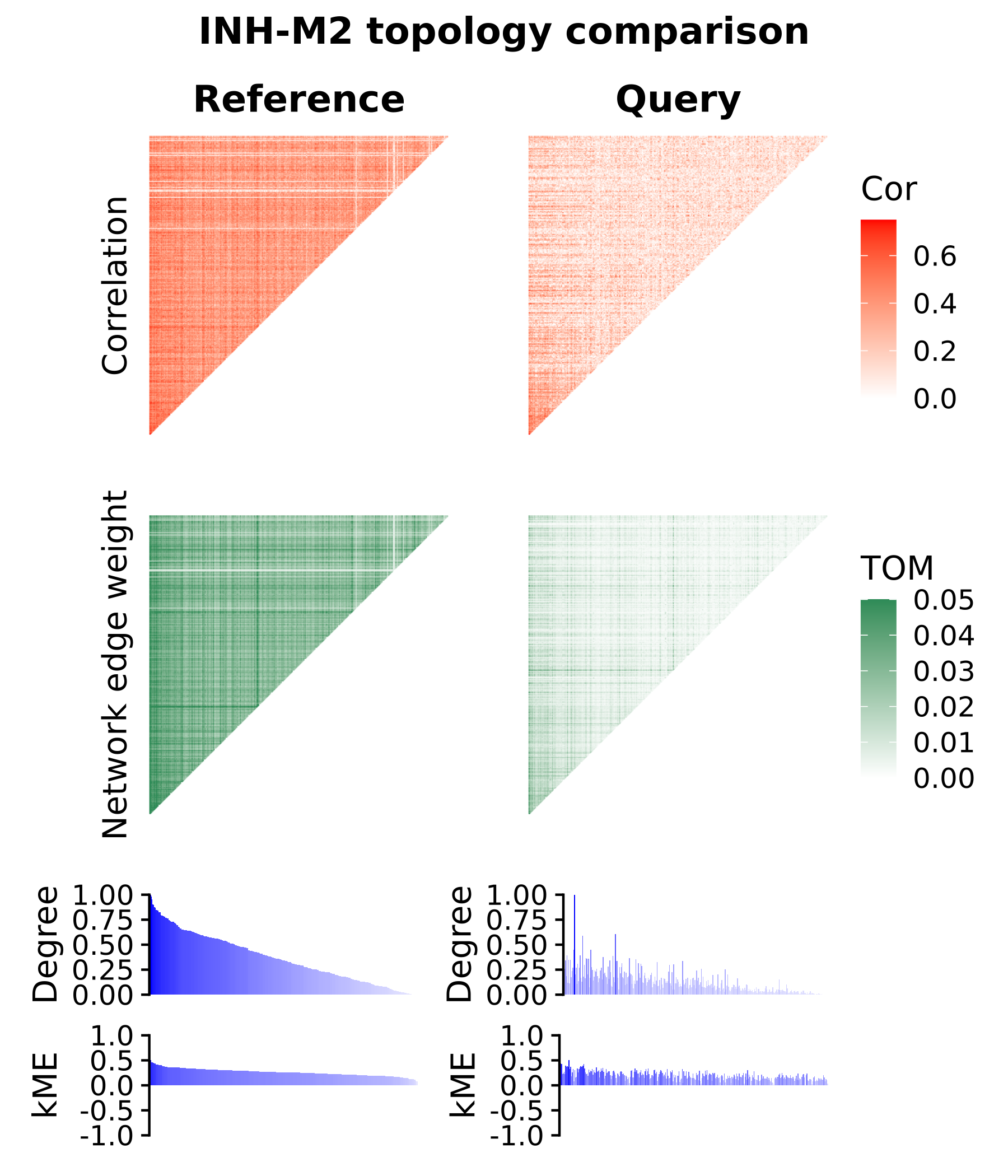
In the module topology plots for module INH-M9, we overall see similar signals in the correlation matrix, the TOM, and in the degrees and kME rankings for each gene. This is in contrast to INH-M2, which was not significantly preserved, where the signal is clearly diminished. These plots effectively show us the differences and similarities in the co-expression network topology that are picked up in the module preservation analysis.