Integrating co-expression and protein-protein interaction networks

Compiled: 24-01-2024

Introduction

Co-expression networks are a useful approach for identifying biological patterns in a transcriptomic dataset in an unsupervised manner. However, interpreting individual co-expression patterns is not always straightforward. What does a strong co-expression between a pair of genes mean? Does gene A regulate gene B? Are they part of the same pathway? Expressed in the same cell type, disease state, timepoint, etc? In this tutorial, we aim to add more interpretability to the co-expression network by integrating it with a protein-protein interaction (PPI) network. This advanced tutorial is inspired by some of our previous works in bulk transcriptomics for human and mouse datasets, but we have updated the code for compatibility with hdWGCNA.

Important Note: Before running the code in this tutorial, you must first perform the standard co-expression network analysis and module identification with hdWGCNA, as shown in our other tutorial.

# single-cell analysis package
library(Seurat)

# plotting and data science packages:
library(tidyverse)
library(cowplot)
library(patchwork)
library(magrittr)
library(patchwork)

# co-expression network analysis packages:
library(WGCNA)
library(hdWGCNA)

# network analysis & visualization package:
library(igraph)

# using the cowplot theme for ggplot
theme_set(theme_cowplot())

# set random seed for reproducibility
set.seed(12345)

# re-load the Zhou et al snRNA-seq dataset
seurat_obj <- readRDS('data/Zhou_control.rds')

Install additional packages

For this analysis, we rely on the Bioconductor package STRINGdb to retrieve the PPI data.

# install STRINGdb
BiocManager::install('STRINGdb')

# load STRINGdb
library(STRINGdb)

Integrating co-expression and PPI networks

Since we already have a co-expression network generated with hdWGCNA, now we need a PPI network. First, we use the R package STRINGdb to set up a PPI network. Here we briefly explain some of the options for initializing the network, but please consult the STRINBdb documentation for further details about using this package. In principle, other PPI resources may be used instead of STRINGdb.

Create the PPI `igraph` object.

In this section, we represent the PPI network using an igraph object. First, we generate a STRINGdb object using the class constructor STRINGdb$new.

version: the STRING version.
species: the species taxonomy ID. Human is 9606, mouse is 10090. For other species, check the NCBI taxonomoy.
score_threshold: the minimum combined interaction score for a PPI to be included in the network.
network_type: the type of network interactions to use. STRING uses both functional and physical interaction data to rank PPIs for the full network, but you can choose to just use one or the other if you wish.

After we initialize the STRINGdb object, we call the function get_graph() to convert it to an igraph object.

# initialize the stringdb
string_db <- STRINGdb$new( 
    version="12.0", species=9606, 
    score_threshold=200, 
    network_type="full", 
    input_directory="" 
)

# retrieve the full PPI graph as an igraph object
ppi <- string_db$get_graph()

Now we have ppi, an igraph object containing the full network of PPIs. Let’s quickly check how many protiens (vertices) and how many PPIs (edges) are in this network.

n_ppis <- length(E(ppi))
n_proteins <- length(V(ppi))
print(paste0("N proteins: ", n_proteins, ' | N PPIs: ', n_ppis))

[1] "N proteins: 19611 | N PPIs: 7533072"

Match protein and gene names

Let’s check how the proteins are named in the PPI network.

head(names(V(ppi)))

[1] "9606.ENSP00000000233" "9606.ENSP00000000412" "9606.ENSP00000001008"
[4] "9606.ENSP00000001146" "9606.ENSP00000002125" "9606.ENSP00000002165"

Currently, the proteins are named using their Ensembl protein IDs with the species taxonomy ID (9606) appended to the front. In order to integrate the PPI network and the co-expression network, we need a common naming convention. To solve this, we will convert these protein IDs to gene names using Ensembl BioMart. Using BioMart, we generated a table with the following attributes:

Gene.stable.ID
Gene.stable.ID.version
Transcript.stable.ID
Transcript.stable.ID.version
Protein.stable.ID
Protein.stable.Id.version
Gene.name

# load the table from BioMart
ens_df <- read.table('data/ensembl_Grch38_gene_protein.txt', sep='\t', header=1)
head(ens_df)

Gene.stable.ID	Gene.stable.ID.version	Transcript.stable.ID	Transcript.stable.ID.version	Protein.stable.ID	Protein.stable.ID.version	Gene.name
ENSG00000210049	ENSG00000210049.1	ENST00000387314	ENST00000387314.1			MT-TF
ENSG00000211459	ENSG00000211459.2	ENST00000389680	ENST00000389680.2			MT-RNR1
ENSG00000210077	ENSG00000210077.1	ENST00000387342	ENST00000387342.1			MT-TV
ENSG00000210082	ENSG00000210082.2	ENST00000387347	ENST00000387347.2			MT-RNR2
ENSG00000209082	ENSG00000209082.1	ENST00000386347	ENST00000386347.1			MT-TL1
ENSG00000198888	ENSG00000198888.2	ENST00000361390	ENST00000361390.2	ENSP00000354687	ENSP00000354687.2	MT-ND1

Our Seurat object and the co-expression network use gene names, so we will convert the protein names in the PPI network to gene names.

IMPORTANT NOTE: This approach is sufficient for the purpose of the tutorial, but ideally we should convert the gene names in the Seurat object to Ensembl Gene IDs, and then match the Ensembl Protein IDs with the Ensembl Gene IDs because Ensembl IDs are more stable/robust than gene names.

# remove the Taxonomy ID from the protein names
ppi <- igraph::set_vertex_attr(
    ppi, 'name', 
    value=stringr::str_replace(names(V(ppi)), '9606.', '')
)

# subset the table for genes that are in the Seurat obj & have a corresponding 
# protein entry in the PPI network
ens_df <- subset(
    ens_df, 
    Gene.name %in% rownames(seurat_obj) & 
    Protein.stable.ID %in% names(V(ppi))
)

# subset the PPI network to just proteins found in our Ensembl data
ppi <- igraph::subgraph(
    ppi,
    vids = unique(ens_df$Protein.stable.ID)
)

# match the protein names w/ gene names, update the PPI network
ix <- match(names(V(ppi)), ens_df$Protein.stable.ID)
ppi <- igraph::set_vertex_attr(
    ppi, 'name', 
    value=ens_df$Gene.name[ix]
)
head(names(V(ppi)))

[1] "ARF5"    "M6PR"    "FKBP4"   "CYP26B1" "NDUFAF7" "FUCA2"

Combine the co-expression and PPI networks

Now that we have converted the protein IDs to gene names, we subset the PPI to match the same genes as the co-expression network. We also subset the co-expression network (Topological Overlap Matrix, TOM) to match the PPI.

# keep genes that are in the co-expression network and in the PPI network
keep_genes <- GetWGCNAGenes(seurat_obj)
keep_genes <- keep_genes[keep_genes %in% names(V(ppi))]

# subset the PPI network
ppi <- igraph::subgraph(
    ppi,
    vids = keep_genes
)

# get the adjacency matrix representation of the PPI and
# binarize the matrix so 0 means no PPI, 1 means PPI 
ppi_mat <- igraph::as_adjacency_matrix(ppi, sparse=TRUE)
ppi_mat[ppi_mat > 0] <- 1

# get the coex network (TOM), 
TOM <- GetTOM(seurat_obj)
TOM <- TOM[rownames(ppi_mat), colnames(ppi_mat)]

Finally, we will perform an element-wise multiplication of the co-expression network by the binarized PPI network. This means the co-expression information will be retained only if there is evidence of a PPI for a particular gene pair.

# perform element-wise multiplicaiton of the TOM by the PPIs network 
# to only retain gene-gene links supported by PPIs
TOM_ppi <- TOM * as.vector(ppi_mat)

We can visually compare the original co-expression network with the integrated network using the function ModuleTopologyHeatmap. This function simply plots a heatmap of the network adjacency matrix for a particular module.

# get modules and from the seurat obj
modules <- GetModules(seurat_obj) %>% 
  subset(module != 'grey' & gene_name %in% keep_genes) %>%  
  mutate(module = droplevels(module))
mods <- levels(modules$module)

# get module colors for plotting 
mod_colors <- dplyr::select(modules, c(module, color)) %>% distinct()
mod_cp <- mod_colors$color; names(mod_cp) <- as.character(mod_colors$module)

# select the module to plot
cur_mod <- 'INH-M9'

# plot the original co-expression network 
tmp <- ModuleTopologyHeatmap(
    seurat_obj,
    mod = cur_mod,
    matrix = TOM,
    matrix_name = 'TOM',
    order_by = 'kME',
    high_color = mod_cp[cur_mod],
    type = 'unsigned',
    return_genes = TRUE # select this option to get the gene order
) 

# get the plot from the output list
p1 <- tmp[[1]] + ggtitle('Co-expression only') + NoLegend()

# get the gene order from the output list
gene_list <- tmp[[2]]

# plot the integrated network
p2 <- ModuleTopologyHeatmap(
    seurat_obj,
    mod = cur_mod,
    matrix = TOM_ppi,
    matrix_name = 'TOM',
    order_by = 'kME',
    high_color = mod_cp[cur_mod],
    type = 'unsigned',
    plot_max = tmp$plot_max,
    genes_order = gene_list
) + ggtitle('Co-expression + PPI')

# combine with patchwork
(p1 | p2) + plot_annotation(title =cur_mod) & theme(plot.title=element_text(hjust=0.5))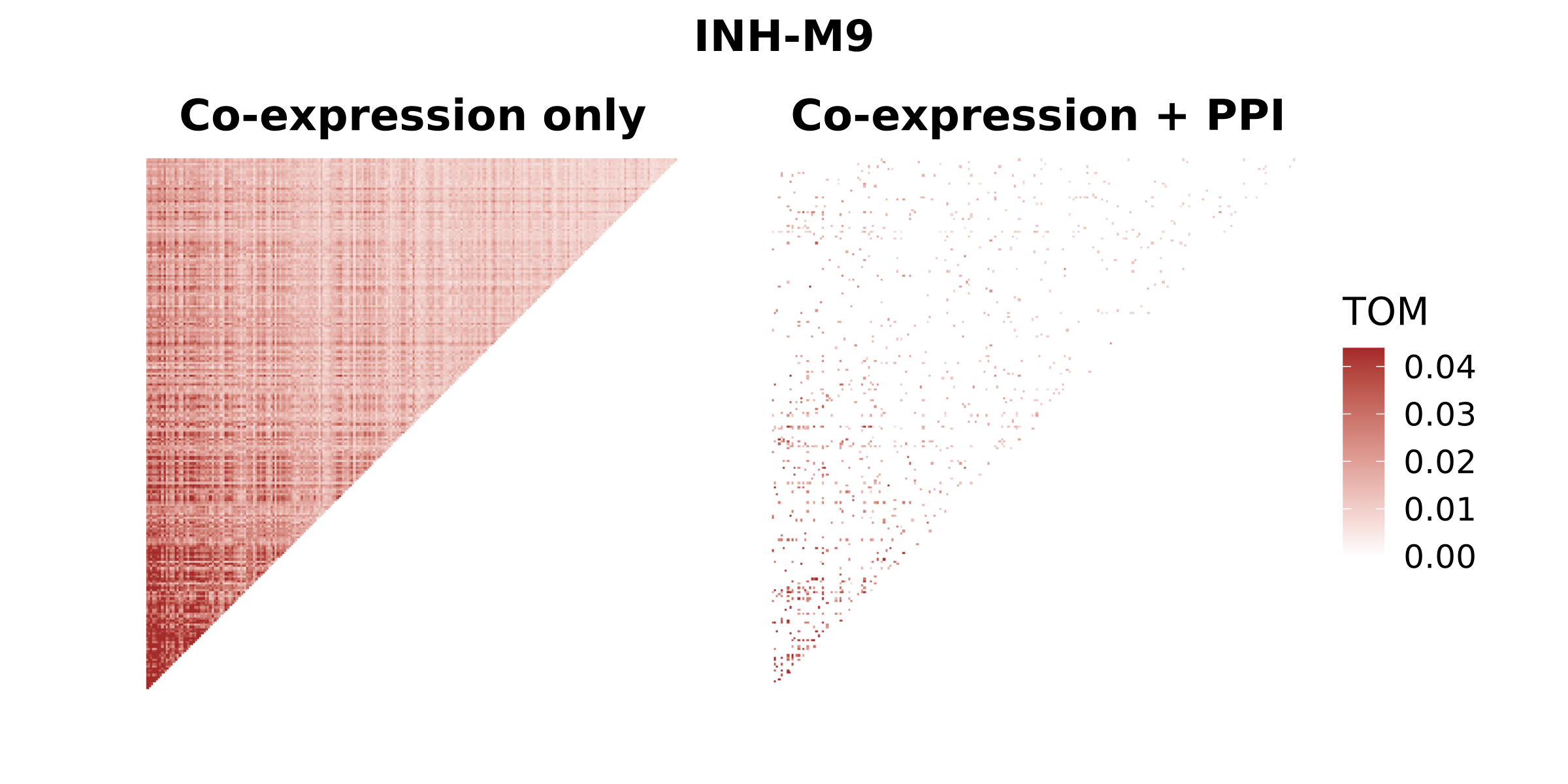

In this heatmap, we can easily see that many of the gene-gene edges in the co-expression network are missing in the integrated network. This is expected, and it is because the integrated network only contains gene-gene edges where there is evidence of a protein-protein interaction.

Identifying hub genes in the integrated network

Network hub genes are genes with strong connections in a co-expression module, and they are typically interesting candidates for further analysis. However, since we now have a different network only containing gene-gene links with PPI support, the connectivity of the network has changed substntially, and therefore the hub genes have likely changed as well.

In this section, we calculate the connectivity of each gene in the integrated network for one module, and compare this to the eigengene-based connectivity (kME) which we typically use to identify module hub genes. We will then make a scatter plot comparing these two measures of connectivity for each gene, and we will label the top hub genes with evidence from both the original co-expression network and the integrated network.

# get the list of genes in this module 
cur_genes <- modules %>% subset(module == cur_mod) %>% .$gene_name

# get the kME for this module
kme_df <- GetHubGenes(seurat_obj, n_hubs=Inf) %>%
    subset(gene_name %in% cur_genes)
rownames(kme_df) <- kme_df$gene_name

# subset TOM for genes in this module
cur_TOM_ppi <- TOM_ppi[cur_genes,cur_genes] 
cur_TOM_ppi[lower.tri(cur_TOM_ppi)] <- 0 

# cast from from matrix to long dataframe, remove self-links
cur_TOM_df <- reshape2::melt(cur_TOM_ppi) %>% subset(Var1 != Var2)

# calculate degree for each gene and arrange by degree
ppi_degree <- cur_TOM_df %>% 
    dplyr::group_by(Var1) %>% 
    dplyr::summarise(degree = sum(value)) %>%
    dplyr::mutate(weighted_degree = degree / max(degree)) %>%
    dplyr::arrange(-degree) %>% 
    dplyr::rename(gene_name = Var1) %>%
    as.data.frame() 
rownames(ppi_degree) <- ppi_degree$gene_name

# combine into 1 table:
kme_df$ppi_degree <- ppi_degree[kme_df$gene_name, 'degree']

#------------------------------------------------------#
# Plot kME vs PPI connectivity
#------------------------------------------------------#

# what are the top n genes (hub genes) by kME vs by ppi? 
n_genes <- 25
top_kme <- kme_df %>% slice_max(order_by=kME, n=n_genes) %>% .$gene_name
top_ppi <- kme_df %>% slice_max(order_by=ppi_degree, n=n_genes) %>% .$gene_name

# get the genes common to both groups
top_both <- intersect(top_kme, top_ppi)
df_kme <- subset(kme_df, gene_name %in% top_kme & !(gene_name %in% top_both))
df_ppi <- subset(kme_df, gene_name %in% top_ppi & !(gene_name %in% top_both))
df_both <- subset(kme_df, gene_name %in% top_both)

# define the x and y intercepts for lines showing the hub gene cutoff
v_line <- min(df_kme$kME)
h_line <- min(df_ppi$ppi_degree)

# other plotting parameters
point_size <- 2
cur_color <- mod_cp[cur_mod]

# scatter plot comparing connectivity
p <- kme_df %>% subset(!(gene_name %in% c(top_kme, top_ppi))) %>%
    ggplot(aes(x = kME, y = ppi_degree)) + 
    geom_point(color=cur_color, size=point_size/2) + 
    geom_vline(xintercept=v_line, color='lightgrey', linetype = 'dashed', size=0.5) +
    geom_hline(yintercept=h_line, color='lightgrey', linetype = 'dashed', size=0.5) +
    geom_point(
        data = df_kme, size=point_size,
        fill = cur_color, color = cur_color, shape = 25,
        size=point_size
    ) + 
    geom_point(
        data = df_ppi, size=point_size,
        fill = cur_color, color = cur_color, shape = 24
    ) + 
    geom_point(
        data = df_both, size=point_size*1.5,
        fill = cur_color, color='black', shape=23
    ) + 
    geom_text_repel(
        data = df_both,
        mapping = aes(label=gene_name), color='black'
    ) +
    xlab('Intramodular connectivity (kME)') + 
    ylab('Intramodular PPI connectivity (degree)') + 
    theme(
        panel.border=element_rect(color='black', fill=NA, linewidth=0.5),
        axis.line.x=element_blank(),
        axis.line.y=element_blank()
    ) 

p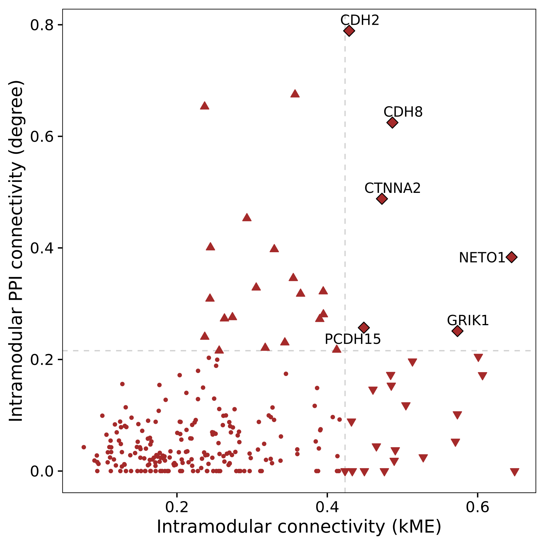

This plot shows the genes that are considered hub genes for the original co-expression network (bottom right, downwards triangle), in the integrated network (upper left, upwards triangle), and in both networks (upper right, diamonds). Among 25 hub genes for each network type, there are 6 in common. This approach effectively narrows down the genes of interest for a particular module by requiring external support for connectivity based on an orthogonal data source, in this case the STRINGdb PPI network.

Visualizing the integrated network

Here we use tidygraph and ggraph to visualize the integrated network. This section is similar to our network visualization tutorial, please consult this tutorial for more information about custom network plots.

# cast the network from wide to long format
graph <- cur_TOM_ppi %>% 
    reshape2::melt() %>% 
    dplyr::rename(gene1 = Var1, gene2 = Var2, weight=value) %>%
    subset(weight > 0) %>%
    igraph::graph_from_data_frame() %>%
    tidygraph::as_tbl_graph(directed=FALSE) %>% 
    tidygraph::activate(nodes)

# add the module name to the graph:
V(graph)$module <- modules[V(graph)$name,'module']

# add the hub gene status and connectivity
V(graph)$hub <- ifelse(V(graph)$name %in% top_both, V(graph)$name, "")
V(graph)$kME <- kme_df[V(graph)$name, 'kME']
V(graph)$ppi_degree <- kme_df[V(graph)$name, 'ppi_degree']

lay <- ggraph::create_layout(graph, layout_nicely(graph))
lay <- ggraph::create_layout(graph, layout_with_graphopt(graph))

p <- ggraph(lay) + 
  geom_edge_link(aes(alpha=scale01(weight)), color='darkgrey') + 
  geom_node_point(aes(color=module, size=ppi_degree)) +
  geom_node_point(
    data=subset(lay, hub != ''), 
    aes(fill=module, size=ppi_degree), color='black', shape=21
  ) +
  scale_colour_manual(values=mod_cp) +
  scale_fill_manual(values=mod_cp) +
  scale_edge_colour_manual(values=mod_cp) +
  geom_node_label(aes(label=hub), repel=TRUE, max.overlaps=Inf, fontface='italic') +
  NoLegend() + 
  ggtitle(paste0(cur_mod, " integrated network")) + 
  theme(
    plot.title = element_text(hjust=0.5)
  )

p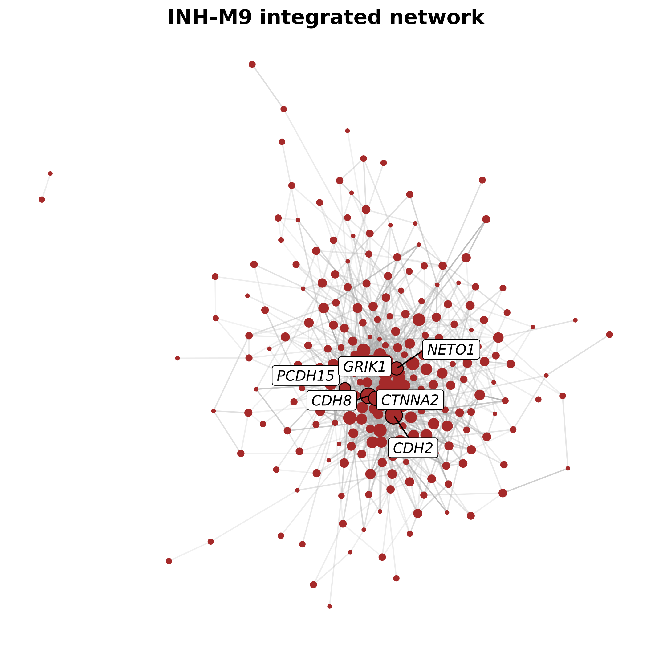

We can repeat this process for all modules in the co-expression network.

Click to see code

plot_list <- list()
for(cur_mod in mods){

    print(cur_mod)

    # get the list of genes in this module 
    cur_genes <- modules %>% subset(module == cur_mod) %>% .$gene_name

    # get the kME for this module
    kme_df <- GetHubGenes(seurat_obj, n_hubs=Inf) %>%
        subset(gene_name %in% cur_genes)
    rownames(kme_df) <- kme_df$gene_name

    # subset TOM for genes in this module
    cur_TOM_ppi <- TOM_ppi[cur_genes,cur_genes] 
    cur_TOM_ppi[lower.tri(cur_TOM_ppi)] <- 0 

    # cast from from matrix to long dataframe, remove self-links
    cur_TOM_df <- reshape2::melt(cur_TOM_ppi) %>% subset(Var1 != Var2)

    # calculate degree for each gene and arrange by degree
    ppi_degree <- cur_TOM_df %>% 
        dplyr::group_by(Var1) %>% 
        dplyr::summarise(degree = sum(value)) %>%
        dplyr::mutate(weighted_degree = degree / max(degree)) %>%
        dplyr::arrange(-degree) %>% 
        dplyr::rename(gene_name = Var1) %>%
        as.data.frame() 
    rownames(ppi_degree) <- ppi_degree$gene_name

    # combine into 1 table:
    kme_df$ppi_degree <- ppi_degree[kme_df$gene_name, 'degree']

    # what are the top n genes (hub genes) by kME vs by ppi? 
    n_genes <- 25
    top_kme <- kme_df %>% slice_max(order_by=kME, n=n_genes) %>% .$gene_name
    top_ppi <- kme_df %>% slice_max(order_by=ppi_degree, n=n_genes) %>% .$gene_name
    top_both <- intersect(top_kme, top_ppi)

    # cast the network from wide to long format
    graph <- cur_TOM_ppi %>% 
        reshape2::melt() %>% 
        dplyr::rename(gene1 = Var1, gene2 = Var2, weight=value) %>%
        subset(weight > 0) %>%
        igraph::graph_from_data_frame() %>%
        tidygraph::as_tbl_graph(directed=FALSE) %>% 
        tidygraph::activate(nodes)

    # add the module name to the graph:
    V(graph)$module <- modules[V(graph)$name,'module']

    # add the hub gene status and connectivity
    V(graph)$hub <- ifelse(V(graph)$name %in% top_both, V(graph)$name, "")
    V(graph)$kME <- kme_df[V(graph)$name, 'kME']
    V(graph)$ppi_degree <- kme_df[V(graph)$name, 'ppi_degree']

    lay <- ggraph::create_layout(graph, layout_nicely(graph))
    lay <- ggraph::create_layout(graph, layout_with_graphopt(graph))

    p <- ggraph(lay) + 
    geom_edge_link(aes(alpha=scale01(weight)), color='darkgrey') + 
    geom_node_point(aes(color=module, size=ppi_degree)) +
    geom_node_point(
        data=subset(lay, hub != ''), 
        aes(fill=module, size=ppi_degree), color='black', shape=21
    ) +
    scale_colour_manual(values=mod_cp) +
    scale_fill_manual(values=mod_cp) +
    scale_edge_colour_manual(values=mod_cp) +
    geom_node_label(aes(label=hub), repel=TRUE, max.overlaps=Inf, fontface='italic', size=3) +
    NoLegend() + 
    ggtitle(paste0(cur_mod)) + 
    theme(
        plot.title = element_text(hjust=0.5)
    )

    plot_list[[cur_mod]] <- p
}

wrap_plots(plot_list, ncol=4)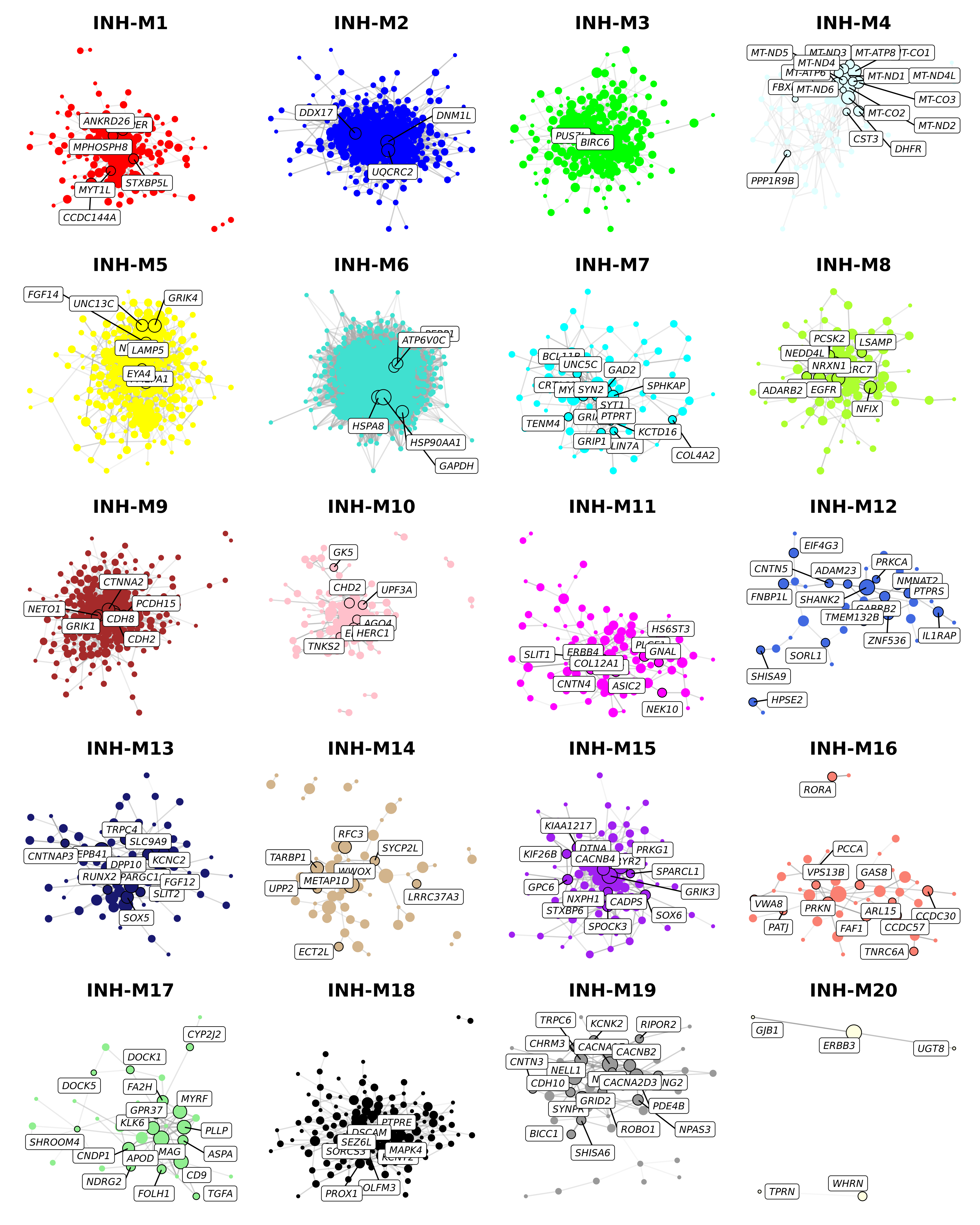

Conclusion

Here we have discussed how to provide further support for the gene-gene links in the co-expression network by integrating with a protein-protein interaction network. If you are interested in further exporing specific gene-gene interactions, there are several external packages that can be explored. For example, both propr and memento are packages that can perform differential analysis of specific gene pairs.