Cross-species and cross-modality analysis

Tutorial Under Construction

In this tutorial, we demonstrate how to use hdWGCNA to project co-expression modules from a reference to a query dataset in certain special cases. Specifically, we project modules from a human snRNA-seq dataset to a human snATAC-seq dataset, a mouse snRNA-seq dataset, and a mouse Visium spatial transcriptomics dataset.

Load the snRNA-seq data and the required libraries:

# single-cell analysis package
library(Seurat)

# plotting and data science packages
library(tidyverse)
library(cowplot)
library(patchwork)

# co-expressi fron network analysis packages:
library(WGCNA)
library(hdWGCNA)

# network analysis & visualization package:
library(igraph)

# using the cowplot theme for ggplot
theme_set(theme_cowplot())

# set random seed for reproducibility
set.seed(12345)

# load the Zhou et al snRNA-seq dataset
seurat_ref <- readRDS('data/Zhou_control.rds')

Project modules from RNA-seq to ATAC-seq

In this section, we project snRNA-seq co-expression modules onto the snATAC-seq dataset from our Nature Genetics paper. This analysis requires a fully processed snRNA-seq dataset that we have run hdWGCNA on, and a fully processed snATAC-seq dataset. For snATAC-seq processing and data formatting, we suggest using Signac, an extension of Seurat for performing single-cell chromatin accessibility analysis. Signac offers several tutorials for processing snATAC-seq data from scratch, and before projecting co-expression modules into snATAC-seq data we need to do the following analysis steps:

• Quality control and filtering.
• Term frequency inverse document frequency (TF-IDF) normalization (RunTFIDF).
• Feature Selection (FindTopFeatures).
• Linear dimensionality reduction (RunSVD).
• Non-linear dimensionality reduction (RunUMAP) for visualizations.
• Group cells into clusters (FindNeighbors and FindClusters).
• Create a gene activity matrix (GeneActivity).

Load snATAC-seq dataset

This following code loads Signac and our snATAC-seq dataset into R.

# single-cell chromatin analysis package:
library(Signac)

# load dataset
seurat_atac <- readRDS('/dfs3b/swaruplab/smorabit/analysis/AD_NucSeq_2019/atac_analysis/all_data/celltype-analysis/data/NucSeq_processed_activity_qc_batch_correct.rds')

To ensure that we loaded the dataset, and that this is indeed a chromatin dataset, we plot the snATAC-seq UMAP and a chromatin accessibility coverage plot for GAD2, an inhibitory neuron marker gene.

Code

# plot the snATAC-seq clusters:
p1 <- DimPlot(seurat_atac, group.by='cell_type', label=TRUE, raster=FALSE) +
   umap_theme() +
   ggtitle('') +
   NoLegend()


p2 <- CoveragePlot(
  object = signac_atac,
  group.by='cell_type',
  region = "GAD2",
  annotation = TRUE, peaks = FALSE, tile = FALSE, links = FALSE
)


png(paste0(fig_dir, 'atac_umap_covplot.png'), width=12, height=4, res=400, units='in')
p1 + p2 +
  plot_layout(widths=c(1,3))
dev.off()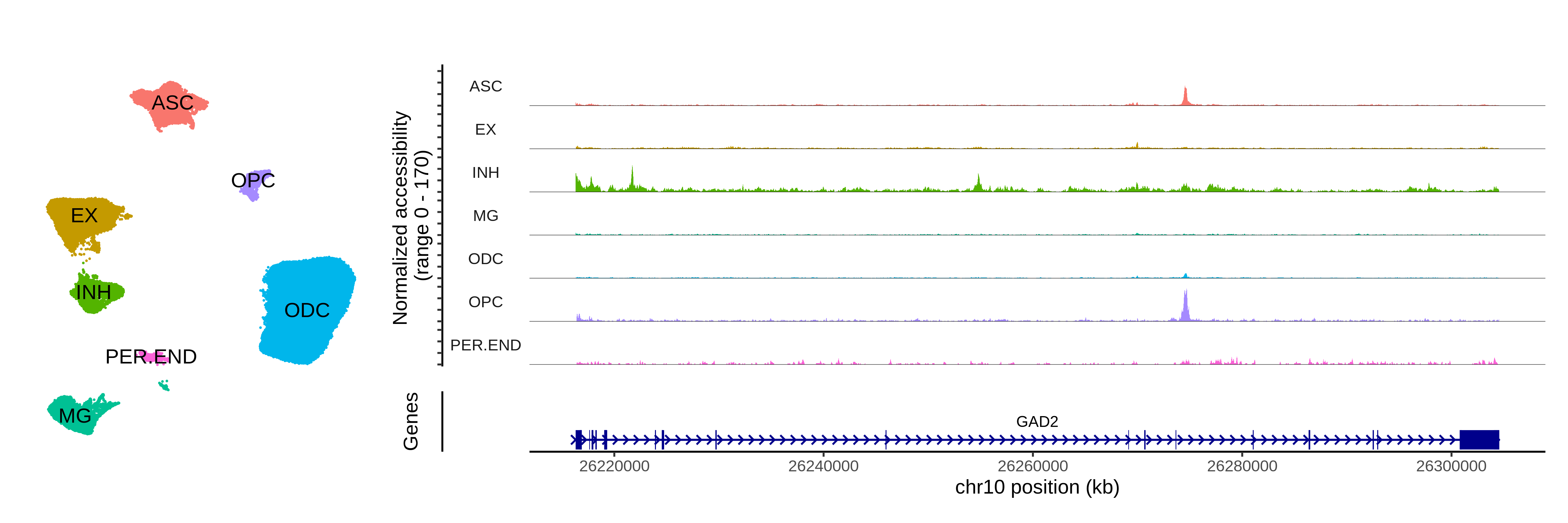

Project modules

In previous examples, the reference and query datasets were both transcriptomics datasets, but here we are trying to investigate co-expression modules in the epigenome using chromatin accessibility data. Here we use the ProjectModules function as we have done before, but we have to ensure that we are using the Gene Activity matrix from the snATAC-seq dataset rather than the chromatin accessibility matrix.

# set assay to RNA (Gene Activity matrix)
DefaultAssay(seurat_atac) <- 'RNA'

# project modules
seurat_atac <- ProjectModules(
  seurat_obj = seurat_atac,
  seurat_ref = seurat_ref,
  group.by.vars = 'Batch',
  wgcna_name = "INH",
  wgcna_name_proj="Zhou_projected"
)

# compute module hub scores for projected modules:
seurat_atac <- ModuleExprScore(
  seurat_atac,
  n_genes = 25,
  method='Seurat'
)

# save the results:
saveRDS(seurat_atac, file='mm2021_atac_hdWGCNA.rds')

Using the gene activity matrix we computed module eigengenes in the snATAC-seq dataset, harmonizing based on the sequencing batch. Additionally, we computed module hub gene expression scores for the projected modules, and now we are ready for visualization and downstream analysis.

Visualize modules in snATAC-seq

Here we will visualize the hub gene expression scores of the projected modules in the snATAC-seq dataset using ModuleFeaturePlot and Seurat’s DotPlot function.

Code

# only show a handful of selected modules
selected_mods <- paste0('INH-M', c(4,5,7,8,9,10))

# make a featureplot of hub scores for each module
plot_list <- ModuleFeaturePlot(
  seurat_atac,
  features='scores',
  order="shuffle",
  module_names = selected_mods
)

# stitch together with patchwork
wrap_plots(plot_list, ncol=3)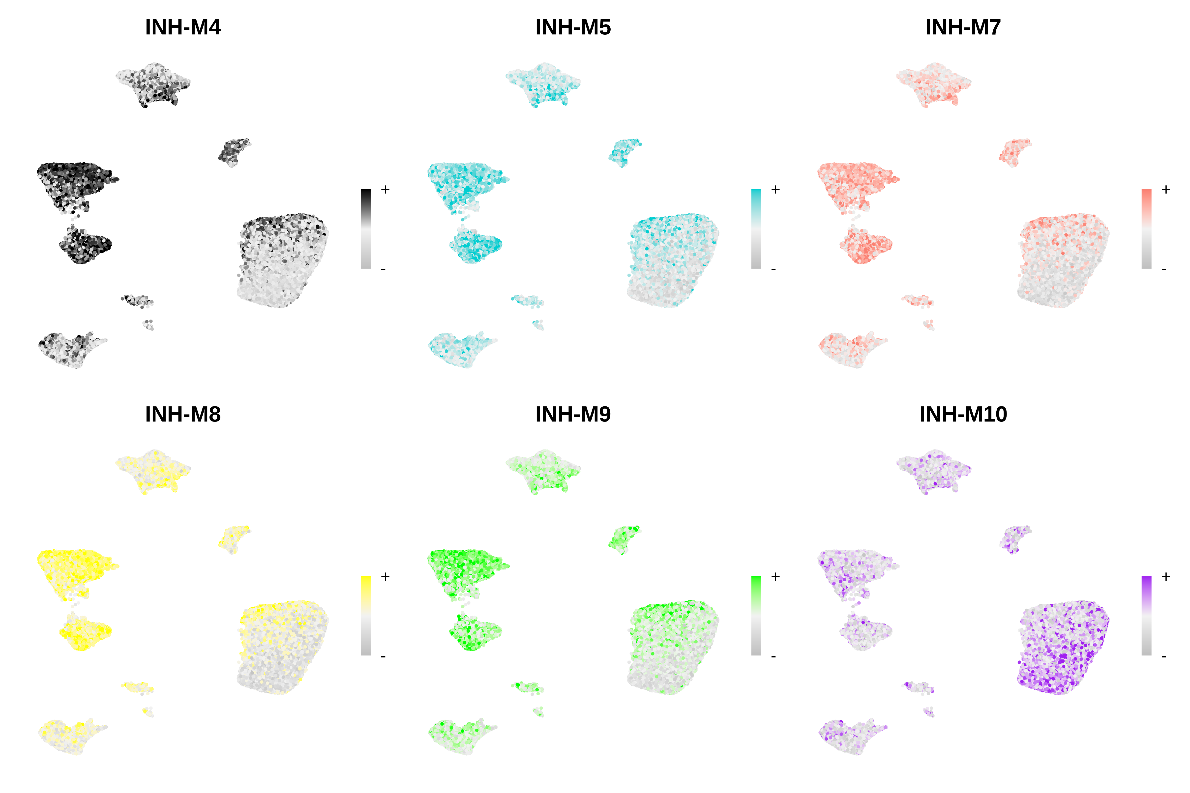

Code

# get the projected hMEs
mod_scores <-  GetModuleScores(seurat_atac)
mod_scores <- mod_scores[,colnames(mod_scores) != 'grey']

# add hMEs to Seurat meta-data:
seurat_atac@meta.data <- cbind(
  seurat_atac@meta.data,
  mod_scores
)

# plot with Seurat's DotPlot function
p <- DotPlot(
    seurat_atac,
    features = colnames(mod_scores),
    group.by = 'cell_type'
)

# flip the x/y axes, rotate the axis labels, and change color scheme:
p <- p +
  RotatedAxis() +
  scale_color_gradient2(high='darkorchid4', mid='grey95', low='seagreen') +
  xlab('') + ylab('')


p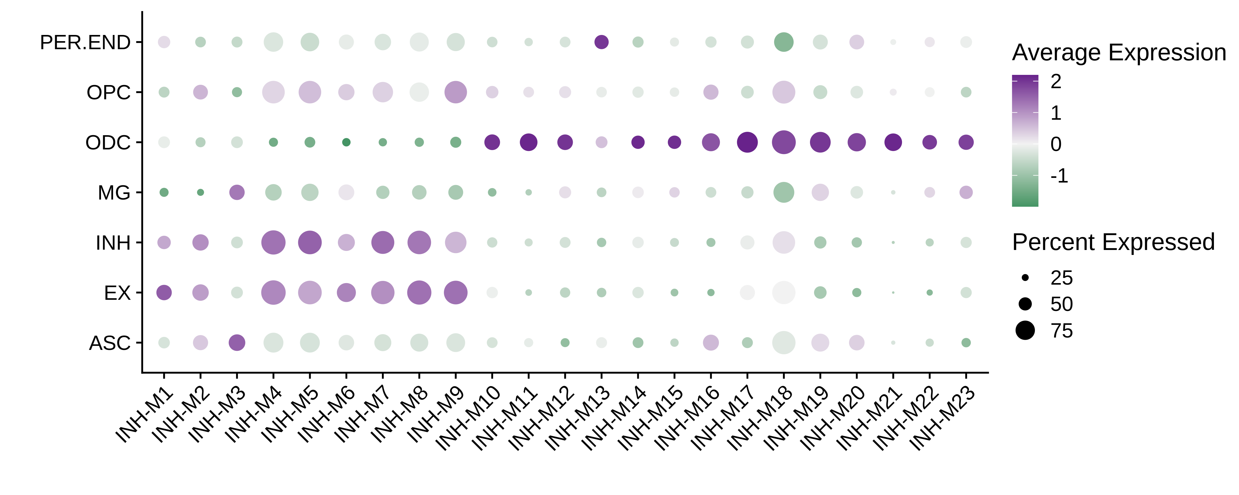

Module preservation in snATAC-seq

In this section, we compute the module preservation statistics for the snATAC-seq dataset. This analysis will tell us which of the co-expression modules are conserved at the epigenome level, and specifically which network properties, such as density or connectiviy, are preserved across modalities. This code is very similar to our previous module preservation analysis, and we do not have to take any specific steps for snATAC-seq here. Note that this code can take a few hours to run on a large query dataset.

# set dat expr for single-cell dataset:
seurat_atac <- SetDatExpr(
  seurat_atac,
  group_name = "INH",
  group.by = "cell_type",
  use_metacells = FALSE
)

# run module preservation function
seurat_atac <- ModulePreservation(
  seurat_atac,
  seurat_ref = seurat_ref,
  name="Zhou-INH",
  verbose=3
)

# save the results again since this step takes a while to run:
saveRDS(seurat_atac, file='mm2021_atac_hdWGCNA.rds')

Now we visualize the results using the PlotModulePreservation function.

Code

# plot the summary stats
plot_list <- PlotModulePreservation(
  seurat_atac,
  name="Zhou-INH",
  statistics = "summary"
)

wrap_plots(plot_list, ncol=2)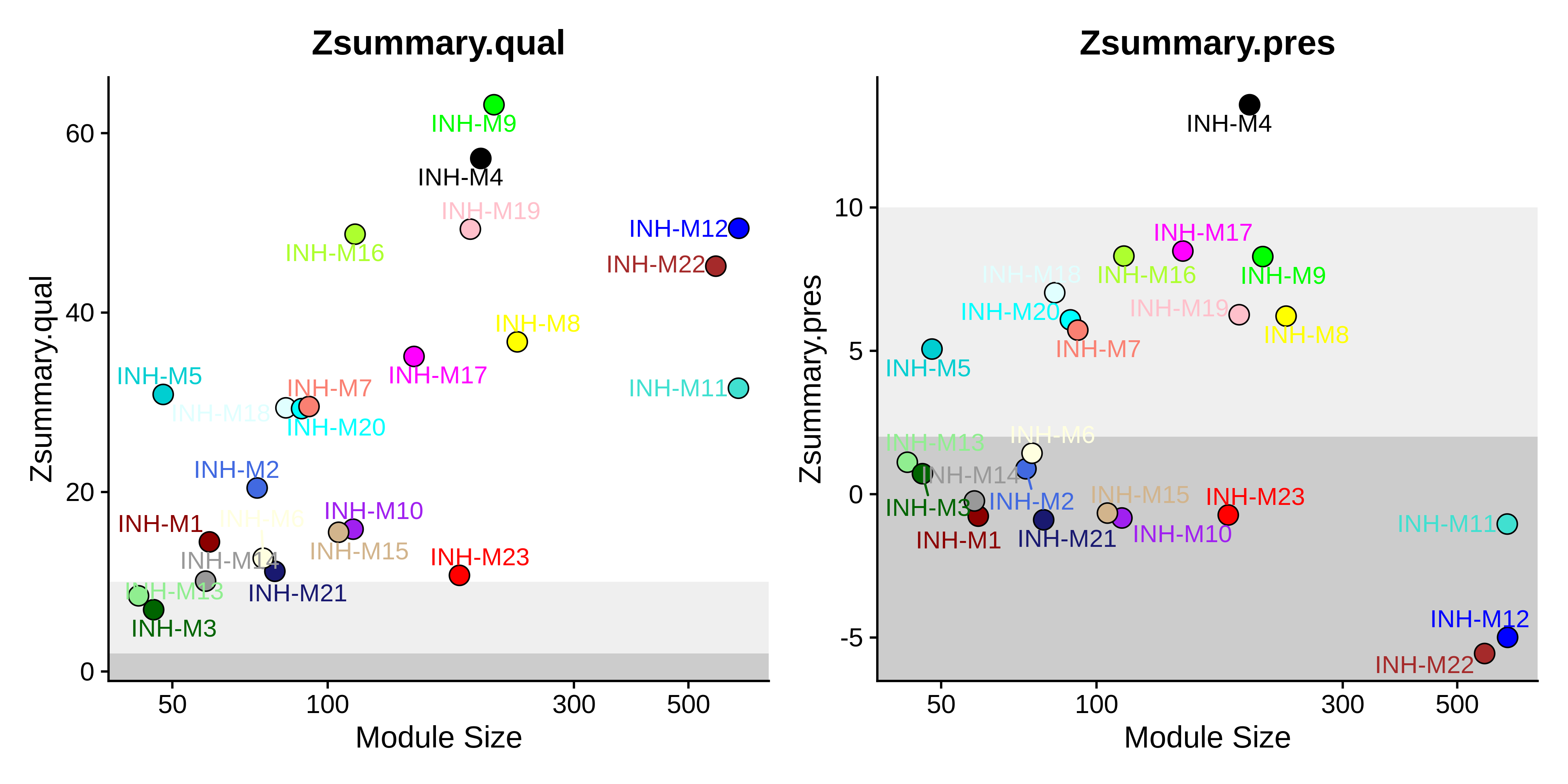

Code

# plot all of the stats togehter
plot_list <- PlotModulePreservation(
  seurat_atac,
  name="Zhou-INH",
  statistics = "all",
  plot_labels=FALSE
)

wrap_plots(plot_list, ncol=6)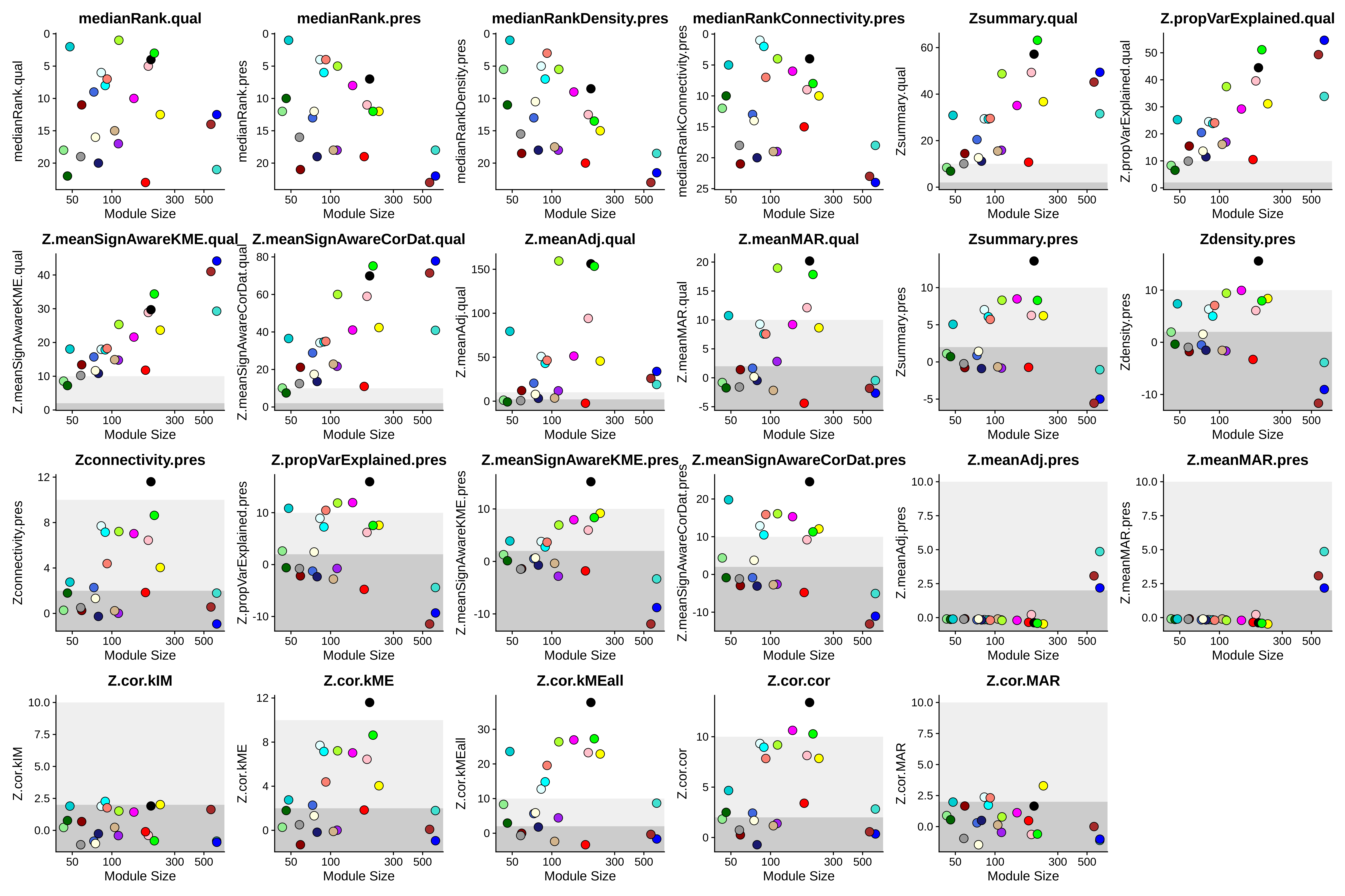

Project modules from hg38 to mm10

# load Zhou et al 5xFAD dataset:
seurat_mouse <- readRDS('/dfs3b/swaruplab/smorabit/analysis/AD_NucSeq_2019/batch_correction/liger/update/mouse_integration/data/zhou_5xFAD_ProcessedSeuratFinal.rds')
seurat_mouse <- subset(seurat_mouse, Cell.Types != 'OTHER')
seurat_mouse$cell_type <- seurat_mouse$Cell.Types
seurat_mouse$cell_type <- ifelse(as.character(seurat_mouse$seurat_clusters) == 13, 'OPC', as.character(seurat_mouse$cell_type))
seurat_mouse$cell_type <- ifelse(as.character(seurat_mouse$seurat_clusters) %in% c(26,27), 'PER', as.character(seurat_mouse$cell_type))


p <- DimPlot(seurat_mouse, group.by = 'cell_type', label = TRUE) +
  umap_theme() +
  NoLegend() + ggtitle('Zhou et al 5xFAD')

png(paste0(fig_dir, 'mouse_umap.png'), units='in', res=400, width=5, height=5)
p
dev.off()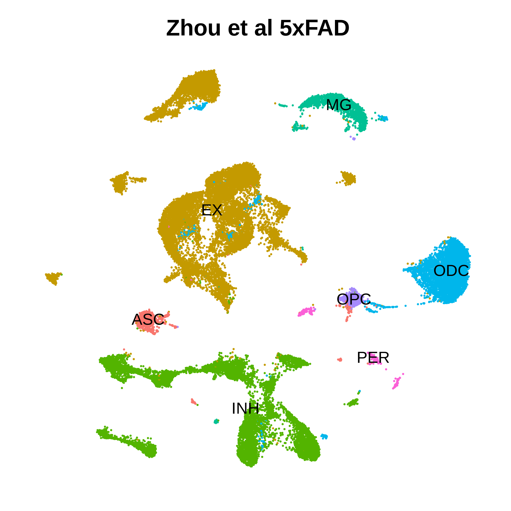

Project modules to 5xFAD data

# load mouse <-> human gene name table:
hg38_mm10_genes <- read.table(
  "/dfs3b/swaruplab/smorabit/resources/hg38_mm10_orthologs_2021.txt",
  sep='\t',
  header=TRUE
)
colnames(hg38_mm10_genes) <-c('hg38_id', 'mm10_id', 'mm10_name', 'hg38_name')
hg38_mm10_genes <- dplyr::select(hg38_mm10_genes, c(hg38_name, mm10_name, hg38_id, mm10_id))


seurat_mouse <- ProjectModules(
  seurat_mouse,
  seurat_ref = seurat_ref,
  gene_mapping=hg38_mm10_genes,
  genome1_col="hg38_name", # genome of reference data
  genome2_col="mm10_name", # genome of query data
  wgcna_name_proj = "Zhou-INH"
)

# compute module hub scores for projected modules:
seurat_mouse <- ModuleExprScore(
  seurat_mouse,
  n_genes = 25,
  method='Seurat'
)

Visualize modules in 5xFAD snRNA-seq

Visualize FeaturePlots

Code

# only show a handful of selected modules
selected_mods <- paste0('INH-M', c(4,5,7,8,9,10))

# make a featureplot of hub scores for each module
plot_list <- ModuleFeaturePlot(
  seurat_mouse,
  features='scores',
  order="order",
  module_names = selected_mods
)

# stitch together with patchwork
png(paste0(fig_dir, 'mouse_featureplot.png'), width=12, height=6, units='in', res=400)
wrap_plots(plot_list, ncol=3)
dev.off()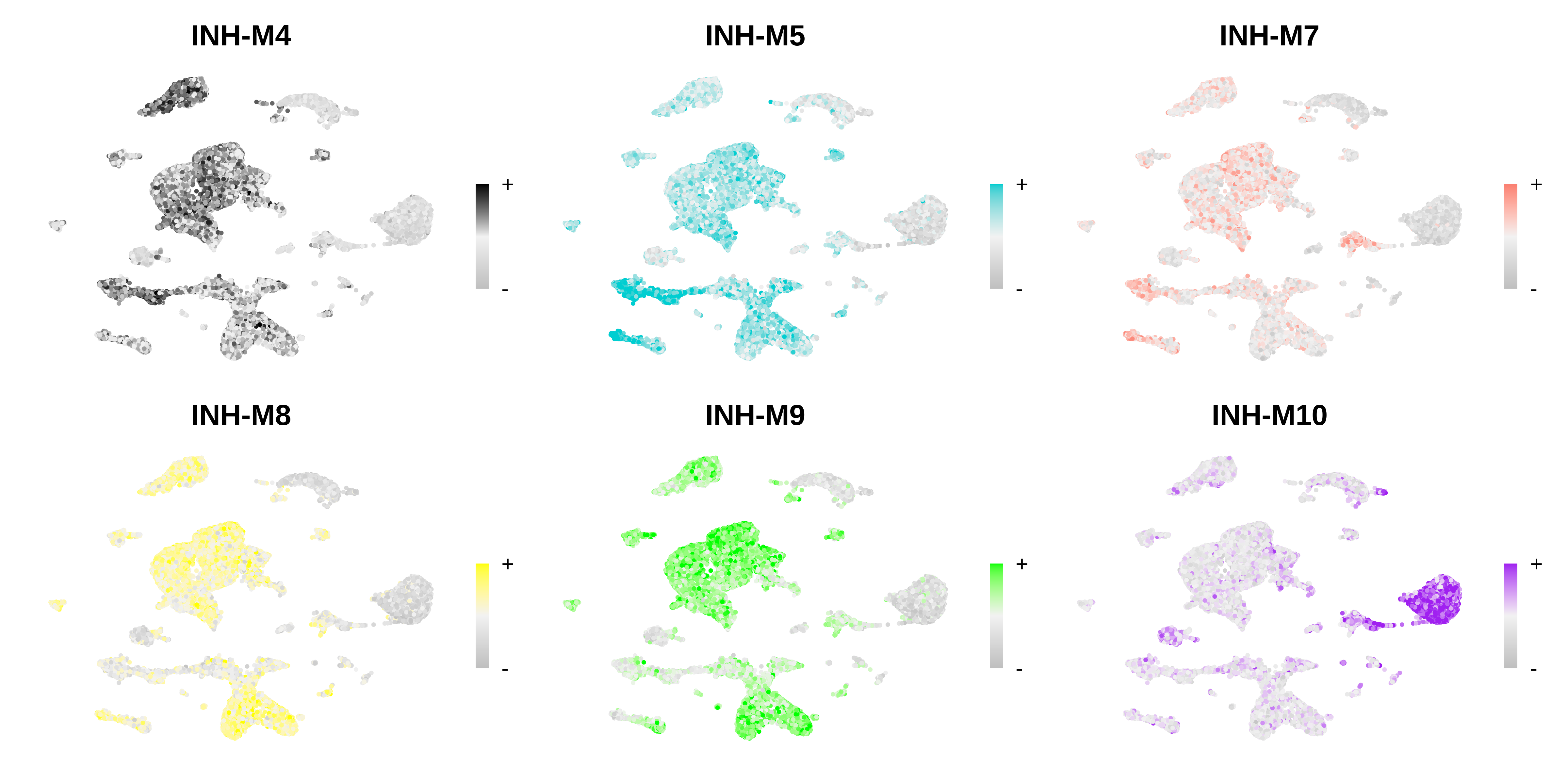

Visualize DotPlots

Code

# get the projected hMEs
mod_scores <-  GetModuleScores(seurat_mouse)
mod_scores <- mod_scores[,colnames(mod_scores) != 'grey']

# add hMEs to Seurat meta-data:
seurat_mouse@meta.data <- cbind(
  seurat_mouse@meta.data,
  mod_scores
)

# plot with Seurat's DotPlot function
p <- DotPlot(
    seurat_mouse,
    features = colnames(mod_scores),
    group.by = 'cell_type'
)

# flip the x/y axes, rotate the axis labels, and change color scheme:
p <- p +
  RotatedAxis() +
  scale_color_gradient2(high='red', mid='grey95', low='blue') +
  xlab('') + ylab('')

png(paste0(fig_dir, 'mouse_dotplot.png'), width=10, height=5, units='in', res=400)
p
dev.off()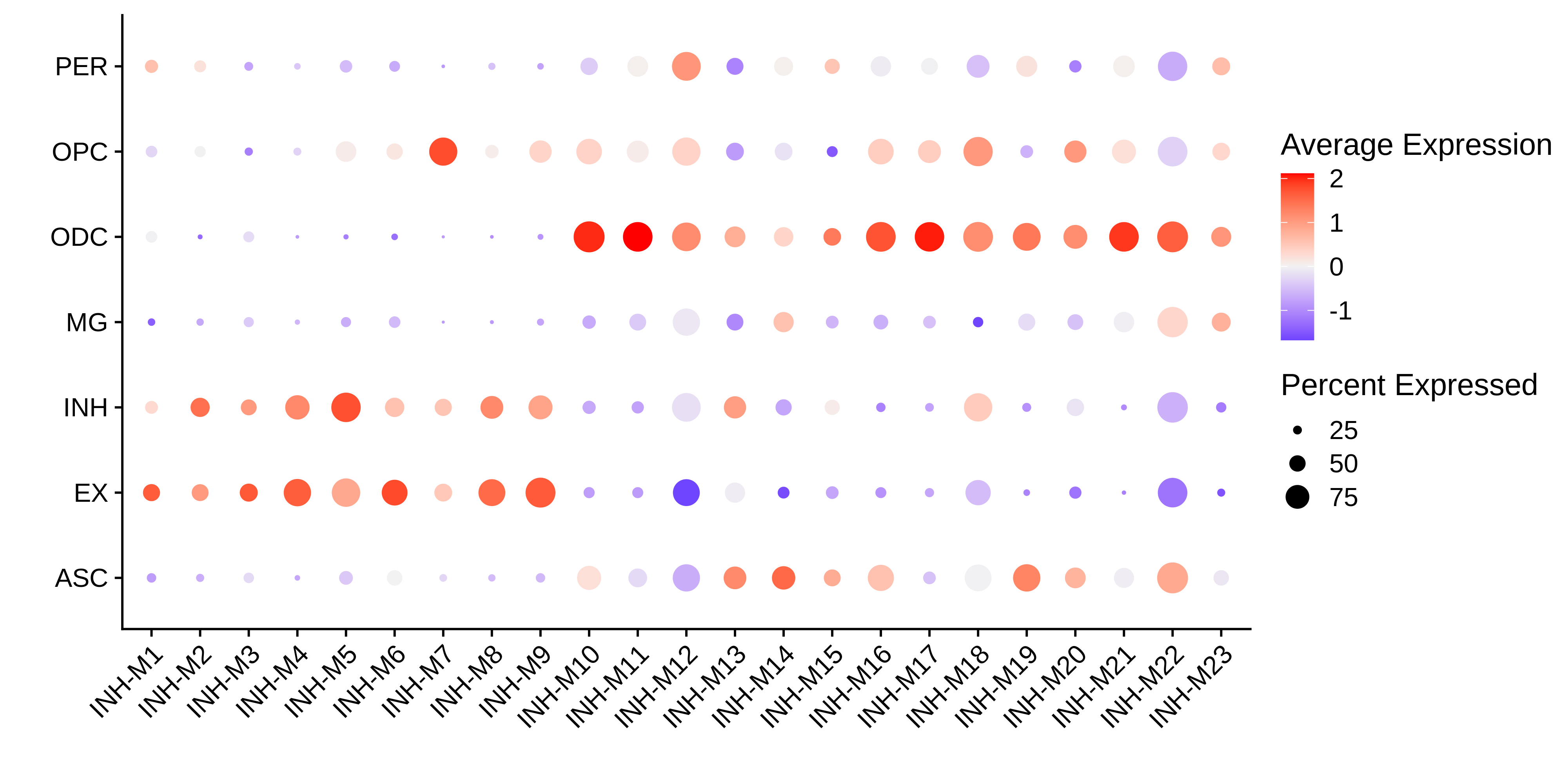

Module preservation

# set dat expr for single-cell dataset:
seurat_mouse <- SetDatExpr(
  seurat_mouse,
  group_name = "INH",
  group.by = "cell_type",
  use_metacells = FALSE
)

# run module preservation function
seurat_mouse <- ModulePreservation(
  seurat_mouse,
  seurat_ref = seurat_ref,
  name="Zhou-INH",
  gene_mapping=hg38_mm10_genes,
  genome1_col="hg38_name", # genome of reference data
  genome2_col="mm10_name", # genome of query data
  verbose=3
)

saveRDS(seurat_mouse, file='../data/5xFAD_zhou_hdWGCNA.rds')

Now we visualize the results using the PlotModulePreservation function.

Code

# plot the summary stats
plot_list <- PlotModulePreservation(
  seurat_mouse,
  name="Zhou-INH",
  statistics = "summary"
)

png(paste0(fig_dir, 'mouse_preservation_summary.png'), width=10, height=5, res=400, units='in')
wrap_plots(plot_list, ncol=2)
dev.off()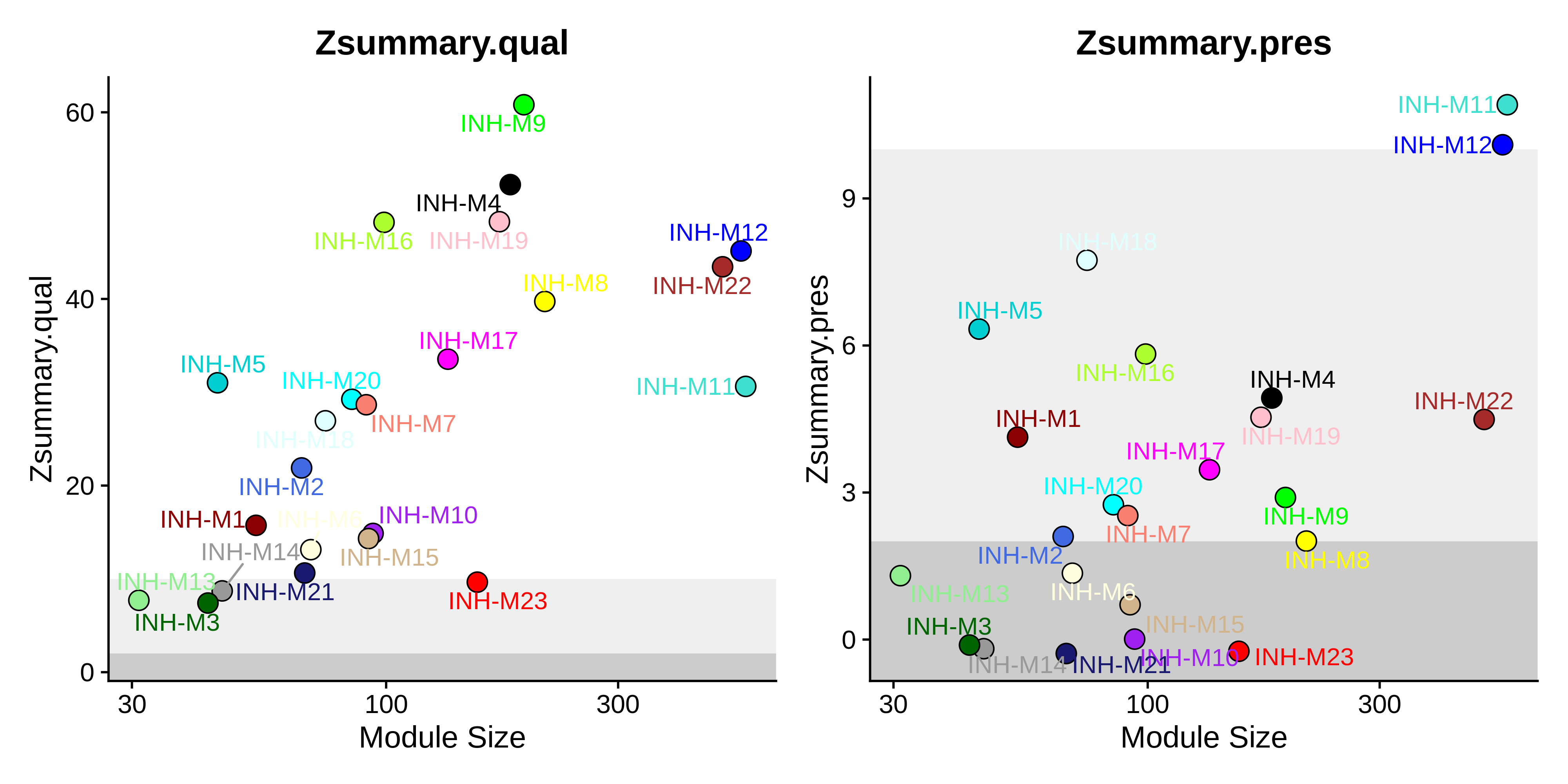

Code

# plot all of the stats togehter
plot_list <- PlotModulePreservation(
  seurat_mouse,
  name="Zhou-INH",
  statistics = "all",
  plot_labels=FALSE
)

png(paste0(fig_dir, 'mouse_preservation_all.png'), width=20, height=20*(2/3), res=400, units='in')
wrap_plots(plot_list, ncol=6)
dev.off()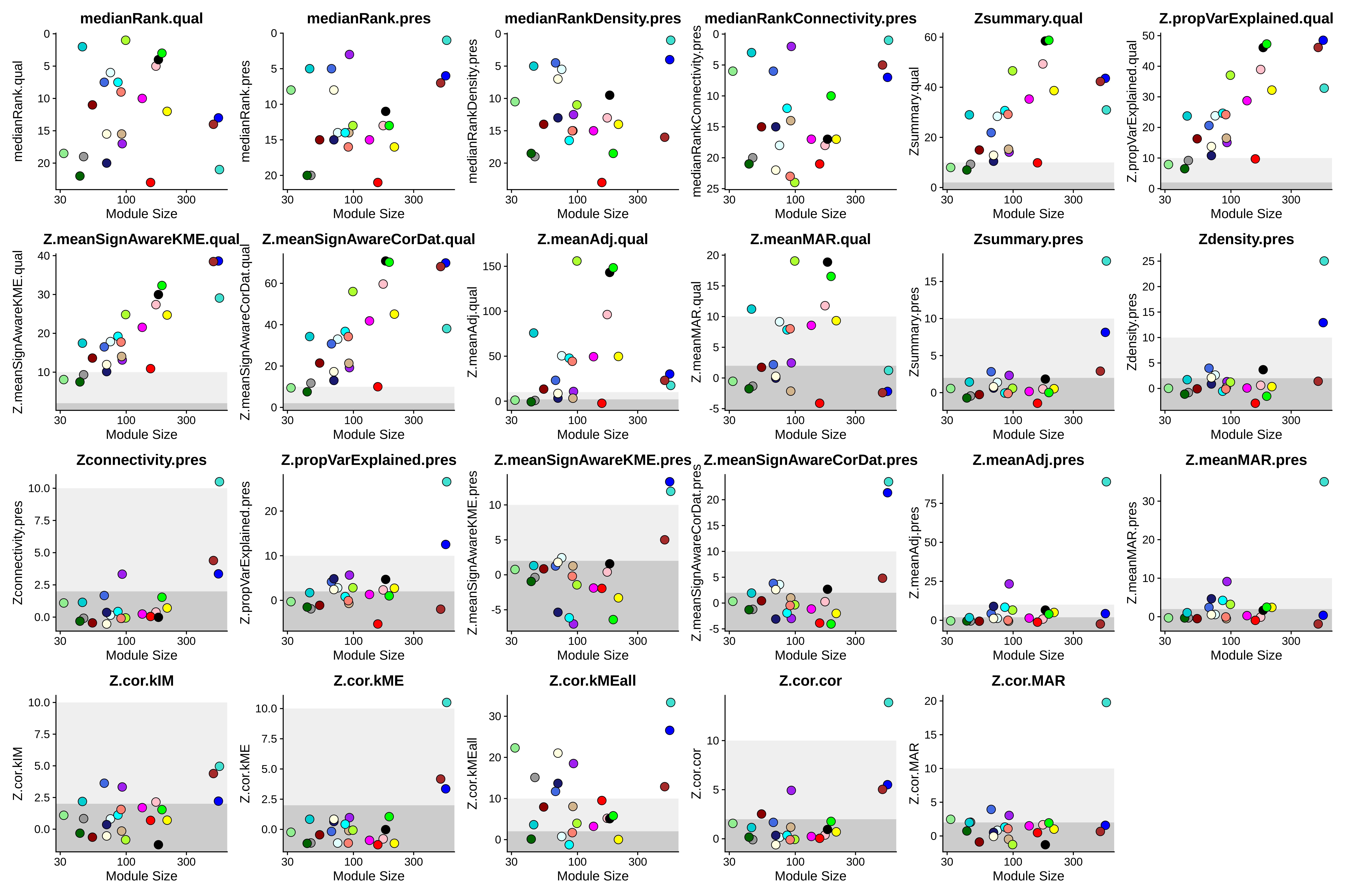

Project modules to visium data

Download and process Visium brain dataset

# load 10X genomics visium dataset
SeuratData::InstallData("stxBrain")
seurat_vis <- SeuratData::LoadData("stxBrain", type = "anterior1")

# process the Visium dataset with Seurat:
seurat_vis <- seurat_vis %>%
  NormalizeData() %>%
  FindVariableFeatures() %>%
  ScaleData() %>%
  RunPCA() %>%
  RunUMAP(dims=1:30) %>%
  FindNeighbors(dims=1:30) %>%
  FindClusters(res=0.75)


p1 <- DimPlot(seurat_vis, reduction = "umap", label = TRUE) +
  umap_theme() +
  NoLegend()

p2 <- SpatialDimPlot(seurat_vis, label = TRUE, label.size = 3) +
  NoLegend()

png(paste0(fig_dir, 'vis_umap.png'), units='in', res=400, width=10, height=5)
p1 | p2
dev.off()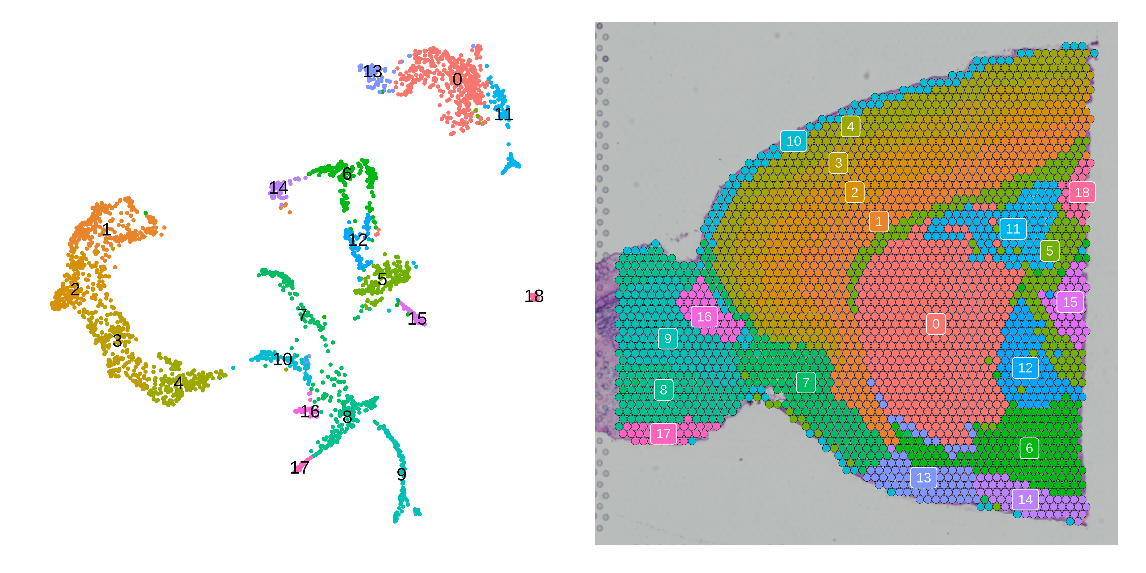

Project modules to visium dataset:

Load the mouse to human gene table

# load mouse <-> human gene name table:
hg38_mm10_genes <- read.table(
  "/dfs3b/swaruplab/smorabit/resources/hg38_mm10_orthologs_2021.txt",
  sep='\t',
  header=TRUE
)
colnames(hg38_mm10_genes) <-c('hg38_id', 'mm10_id', 'mm10_name', 'hg38_name')
hg38_mm10_genes <- dplyr::select(hg38_mm10_genes, c(hg38_name, mm10_name, hg38_id, mm10_id))

Project Modules

seurat_vis <- ProjectModules(
  seurat_vis,
  seurat_ref = seurat_ref,
  gene_mapping=hg38_mm10_genes,
  genome1_col="hg38_name", # genome of reference data
  genome2_col="mm10_name", # genome of query data
  wgcna_name_proj = "Zhou-INH"
)

# compute module hub scores for projected modules:
seurat_vis <- ModuleExprScore(
  seurat_vis,
  n_genes = 25,
  method='Seurat'
)

Spatial Feature Plot:

# get all of the image coordinates for BayesSpace
image_df <- do.call(rbind, lapply(names(seurat_vis@images), function(cur_image){seurat_vis@images[[cur_image]]@coordinates}))

# re-order the rows of image_df to match the seurat_obj
image_df <- image_df[colnames(seurat_vis),]
all.equal(rownames(image_df), colnames(seurat_vis))

# make a spatial "reduction"
image_emb <- as.matrix(image_df[,c('col', 'row')])
colnames(image_emb) <- c("Spatial_1", "Spatial_2")
seurat_vis@reductions$spatial <- CreateDimReducObject(
  image_emb,
  key = 'Spatial'
)



# only show a handful of selected modules
selected_mods <- paste0('INH-M', c(4,5,7,8,9,10))

# make a featureplot of hub scores for each module
plot_list <- ModuleFeaturePlot(
  seurat_vis,
  features='scores',
  order="order",
  module_names = selected_mods,
  reduction='spatial'
)

# stitch together with patchwork
png(paste0(fig_dir, 'visium_featureplot.png'), width=12, height=6, units='in', res=400)
wrap_plots(plot_list, ncol=3)
dev.off()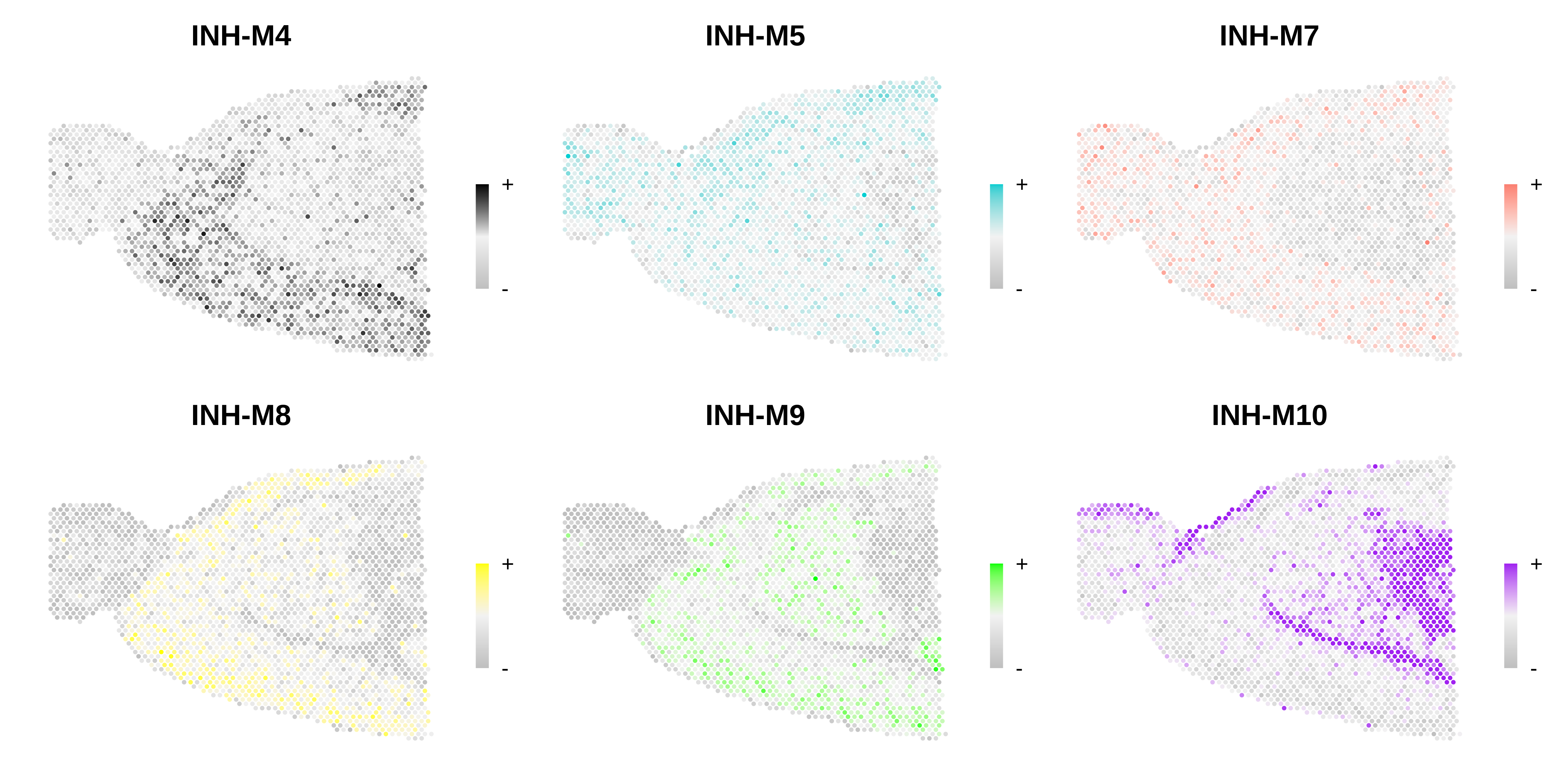

# make a featureplot of hub scores for each module
plot_list <- ModuleFeaturePlot(
  seurat_vis,
  features='scores',
  order="order",
  module_names = selected_mods,
  reduction='umap'
)

# stitch together with patchwork
png(paste0(fig_dir, 'visium_featureplot_umap.png'), width=12, height=6, units='in', res=400)
wrap_plots(plot_list, ncol=3)
dev.off()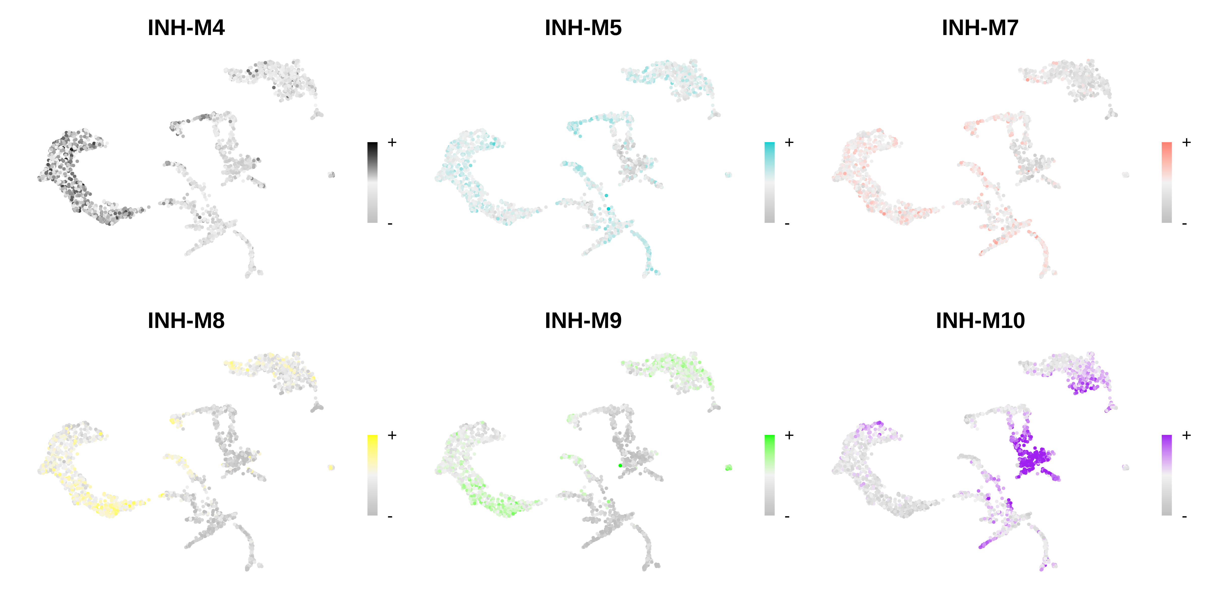

Module preservation in Visium:

# set dat expr for single-cell dataset:
seurat_vis <- SetDatExpr(
  seurat_vis,
  use_metacells = FALSE
)

# run module preservation function
seurat_vis <- ModulePreservation(
  seurat_vis,
  seurat_ref = seurat_ref,
  name="Zhou-INH",
  verbose=3
)

seurat_vis <- ModulePreservation(
  seurat_vis,
  seurat_ref = seurat_ref,
  name="Zhou-INH",
  gene_mapping=hg38_mm10_genes,
  genome1_col="hg38_name", # genome of reference data
  genome2_col="mm10_name", # genome of query data
  verbose=3
)

saveRDS(seurat_vis, file='../data/10x_visium_hdWGCNA.rds')

Now we visualize the results using the PlotModulePreservation function.

Code

# plot the summary stats
plot_list <- PlotModulePreservation(
  seurat_vis,
  name="Zhou-INH",
  statistics = "summary"
)

png(paste0(fig_dir, 'visium_preservation_summary.png'), width=10, height=5, res=400, units='in')
wrap_plots(plot_list, ncol=2)
dev.off()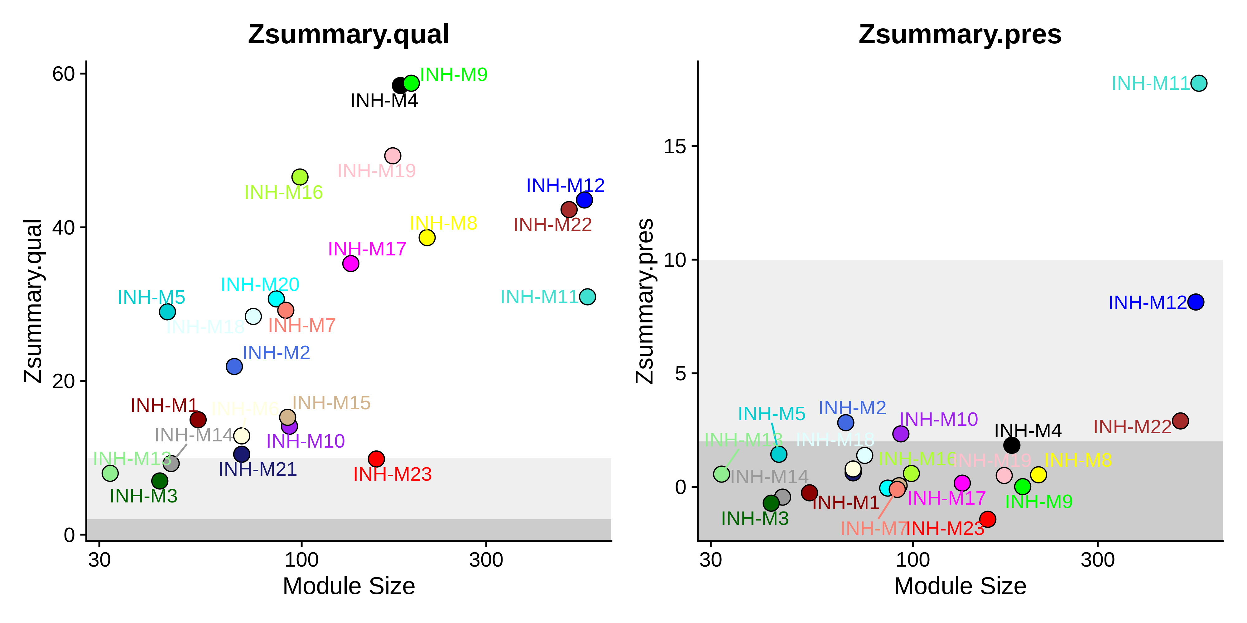

Code

# plot all of the stats togehter
plot_list <- PlotModulePreservation(
  seurat_vis,
  name="Zhou-INH",
  statistics = "all",
  plot_labels=FALSE
)

png(paste0(fig_dir, 'visium_preservation_all.png'), width=20, height=20*(2/3), res=400, units='in')
wrap_plots(plot_list, ncol=6)
dev.off()