Compiled: 07-10-2024
Source: vignettes/ST_basics.Rmd
This tutorial covers the basics of using hdWGCNA to perform co-expression network analysis on transcriptomics (ST) data. Here we primarily focus on sequencing-based approaches like 10X Genomics Visium, (Curio Seeker), and Visium HD. Importantly, there are many different ST approaches resulting in datasets with shared and unique properties which we must consider in our data analysis. For example, some ST protocols have single-cell resolution but only profile a subset of the transcriptome. On the other hand, some ST protocols like Visium and Slide-Seq profile the whole transcriptome. Some ST protocols measure gene expression using sequencing, while others use imaging (i.e. Xenium and CosMX).
Datasets from different ST protocols may require different data analysis steps (i.e. quality control, normalization, clustering), and similarly we take specific steps to perform hdWGCNA for different types of ST. In this tutorial, we demonstrate hdWGCNA using ST datasets from different technologies. First, we use hdWGCNA to analyze a Visium ST dataset containing an anterior and posterior saggital section from the mouse brain. Next, we use hdWGCNA to analyze a Curio Seeker (Slide-Seq) dataset of the mouse hippocampus. Finally, we analyze a similar mouse brain dataset using Visium HD. Overall this tutorial is similar to the hdWGCNA in single-cell data tutorial, and we recommend exploring that tutorial prior to this tutorial.
Load required libraries
First we will load the required R libraries for this tutorial.
# single-cell analysis package
library(Seurat)

# plotting and data science packages
library(tidyverse)
library(cowplot)
library(patchwork)

# co-expression network analysis packages:
library(WGCNA)
library(hdWGCNA)

# enable parallel processing for network analysis (optional)
enableWGCNAThreads(nThreads = 8)

# using the cowplot theme for ggplot
theme_set(theme_cowplot())

# set random seed for reproducibility
set.seed(12345)
10X Visium Dataset
In this section we demonstrate hdWGCNA in ST datasets using a publicly available Visium dataset of the mouse brain.
Load data
Here we use SeuratData to download the mouse brain ST
dataset, and we will process the dataset using Seurat.
Note on SeuratData download
In our own testing, we had difficulty running
InstallData on our institution’s compute cluster, so we ran
these commands locally and then copied the .rds file
containing the Seurat seurat_vhd to the cluster for subsequent
analysis.
# package to install the mouse brain dataset
library(SeuratData)

# download the mouse brain ST dataset (stxBrain)
SeuratData::InstallData("stxBrain")

# load the anterior and posterior samples
brain <- LoadData("stxBrain", type = "anterior1")
brain$region <- 'anterior'
brain2 <- LoadData("stxBrain", type = "posterior1")
brain2$region <- 'posterior'

# merge into one seurat seurat_vhd
seurat_obj <- merge(brain, brain2)
seurat_obj$region <- factor(as.character(seurat_obj$region), levels=c('anterior', 'posterior'))

# save unprocessed seurat_vhd
saveRDS(seurat_obj, file='mouse_brain_ST_unprocessed.rds')
hdWGCNA requires the spatial coordinates to be stored in the
seurat_obj@meta.data slot. Here we extract the image
coordinates for the two samples, merge into a dataframe, and add it into
the seurat_obj@meta.data. Specifically, the
seurat_obj@meta.data must have columns named
row, col, imagerow, and
imagecol (shown below), otherwise the downstream steps will
not work.
IMPORTANT NOTE As of Seurat version 5.1, the image
class was updated from VisiumV1 to VisiumV2.
This changes how Seurat loads Visium data from the
spaceranger outputs. hdWGCNA requires the spot coorinates
in the array, and unfortunately as of Seurat version 5.1 this is no
longer loaded by default with Load10X_Spatial.
spaceranger count outputs a file called tissue_positions.csv,
which contains these coordinates. If you are following with the tutorial
dataset, at this time we recommend using a Seurat version before v5.1.
Please see this
GitHub issue for more information.
Instructions for Seurat versions before v5.1
If you are using a Seurat version older than v5.1, these coordinates are already loaded into the Seurat seurat_vhd, and you can use the following code to add the coordinates to the Seurat metadata slot.
# make a dataframe containing the image coordinates for each sample
image_df <- do.call(rbind, lapply(names(seurat_obj@images), function(x){
  seurat_obj@images[[x]]@coordinates
}))

# merge the image_df with the Seurat metadata
new_meta <- merge(seurat_obj@meta.data, image_df, by='row.names')

# fix the row ordering to match the original seurat seurat_vhd
rownames(new_meta) <- new_meta$Row.names
ix <- match(as.character(colnames(seurat_obj)), as.character(rownames(new_meta)))
new_meta <- new_meta[ix,]

# add the new metadata to the seurat seurat_vhd
seurat_obj@meta.data <- new_meta

head(image_df)
tissue row col imagerow imagecol
AAACAAGTATCTCCCA-1_1 1 50 102 7475 8501
AAACACCAATAACTGC-1_1 1 59 19 8553 2788
AAACAGAGCGACTCCT-1_1 1 14 94 3164 7950
AAACAGCTTTCAGAAG-1_1 1 43 9 6637 2099
AAACAGGGTCTATATT-1_1 1 47 13 7116 2375
AAACATGGTGAGAGGA-1_1 1 62 0 8913 1480Instructions for Seurat versions after v5.1
If you are using a Seurat version v5.1 or newer, these coordinates
are not loaded into the Seurat seurat_vhd by default. We need to load
the tissue_positions.csv file from the
spaceranger output and then add it into the Seurat
seurat_vhd. This section is an example and you need to change the code
to use your own file path. If your Seurat seurat_vhd contains more than
one sample, you will need to repeat this since each sample will have its
own tissue_positions.csv file.
# add barcode column to Seurat obj
seurat_obj$barcode <- colnames(seurat_obj)

# update this with the path for your sample.
tissue_positions <- read.csv('path/to/tissue_positions.csv')
tissue_positions <- subset(tissue_positions, barcode %in% seurat_obj$barcode)

# join the image_df with the Seurat metadata
new_meta <- dplyr::left_join(seurat_obj@meta.data, tissue_positions, by='barcode')

# add the new metadata to the seurat seurat_vhd
seurat_obj$row <- new_meta$array_row
seurat_obj$imagerow <- new_meta$pxl_row_in_fullres
seurat_obj$col <- new_meta$array_col
seurat_obj$imagecol <- new_meta$pxl_col_in_fullres
Now we perform clustering analysis using Seurat.
# normalization, feature selection, scaling, and PCA
seurat_obj <- seurat_obj %>%
  NormalizeData() %>%
  FindVariableFeatures() %>%
  ScaleData() %>%
  RunPCA()

# Louvain clustering and umap
seurat_obj <- FindNeighbors(seurat_obj, dims = 1:30)
seurat_obj <- FindClusters(seurat_obj,verbose = TRUE)
seurat_obj <- RunUMAP(seurat_obj, dims = 1:30)

# set factor level for anterior / posterior
seurat_obj$region <- factor(as.character(seurat_obj$region), levels=c('anterior', 'posterior'))

# show the UMAP
p1 <- DimPlot(seurat_obj, label=TRUE, reduction = "umap", group.by = "seurat_clusters") + NoLegend()
p1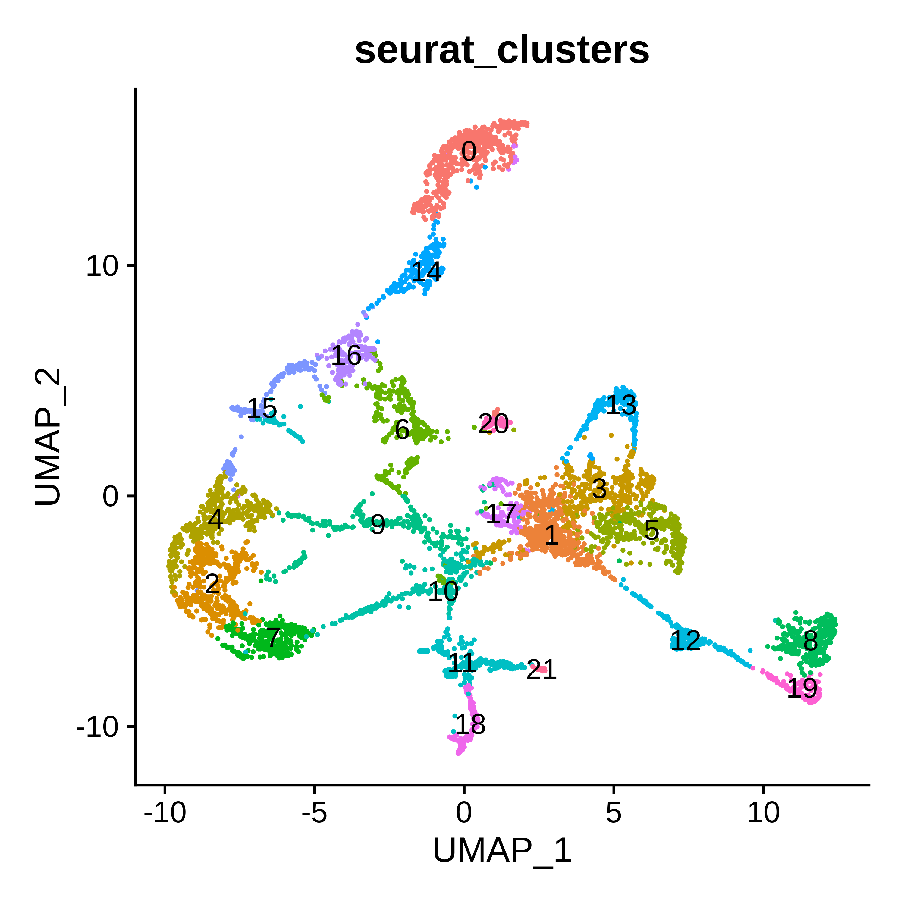
p2 <- SpatialDimPlot(seurat_obj, label = TRUE, label.size = 3)
p2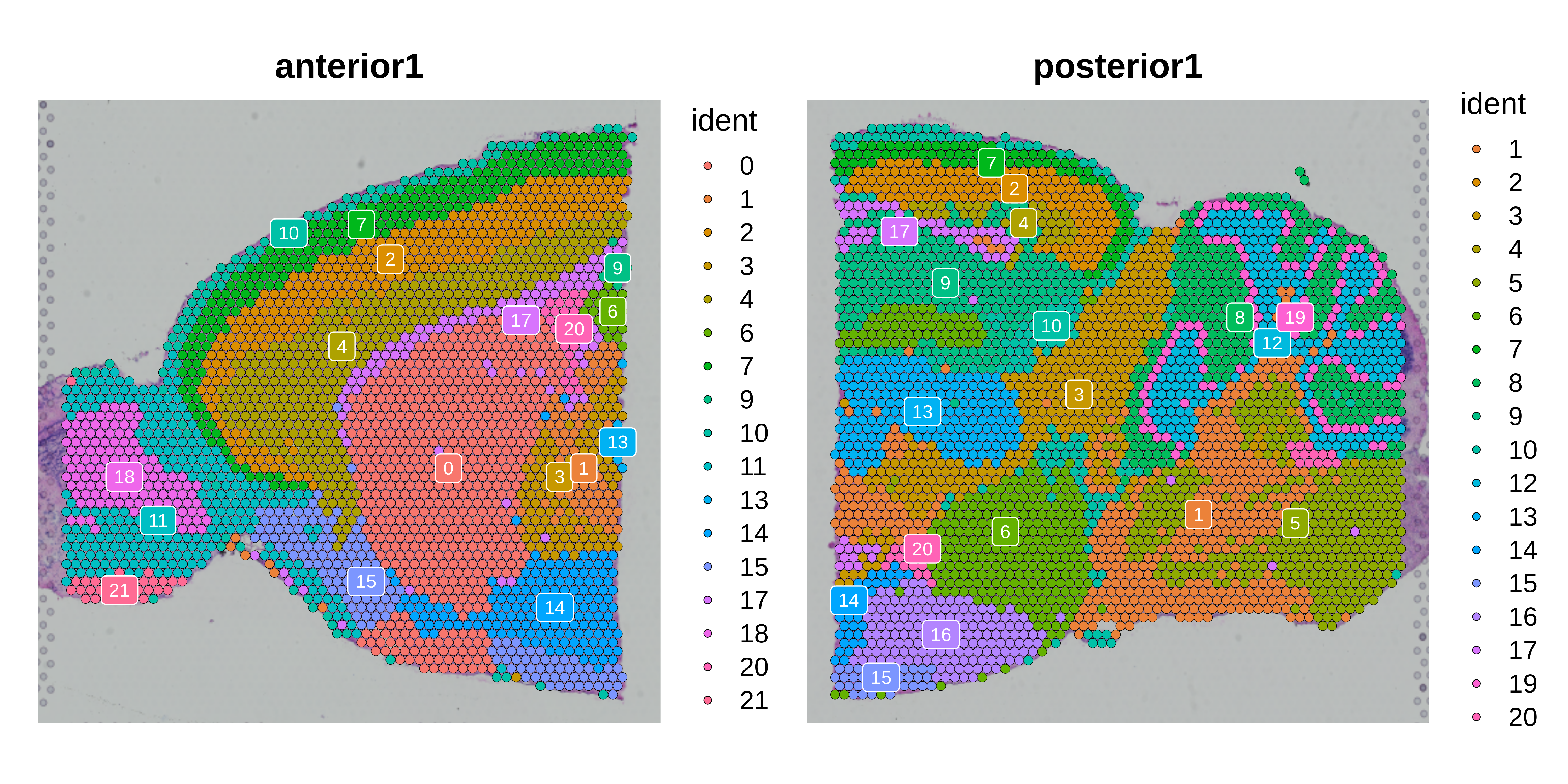
See cluster labels
| seurat_clusters | annotation |
|---|---|
| 0 | Caudoputamen |
| 1 | White matter |
| 2 | Cortex L5 |
| 3 | White matter |
| 4 | Cortex L6 |
| 5 | Medulla |
| 6 | Pons |
| 7 | Cortex L2/3 |
| 8 | Cerebellum molecular layer |
| 9 | Hippocampus |
| 10 | Cortex L1, Vasculature |
| 11 | Olfactory bulb outer |
| 12 | Cerebellum arbor vitae |
| 13 | Thalamus |
| 14 | Nucleus accumbens |
| 15 | Piriform area |
| 16 | Hypothalamums |
| 17 | Fiber tracts |
| 18 | Olfactory bulb inner |
| 19 | Cerebellum granular layer |
| 20 | Ventricles |
| 21 | Olfactory bulb fiber tracts |
# add annotations to Seurat seurat_vhd
annotations <- read.csv('annotations.csv')
ix <- match(seurat_obj$seurat_clusters, annotations$seurat_clusters)
seurat_obj$annotation <- annotations$annotation[ix]

# set idents
Idents(seurat_obj) <- seurat_obj$annotation

p3 <- SpatialDimPlot(seurat_obj, label = TRUE, label.size = 3)
p3 + NoLegend()
Construct metaspots
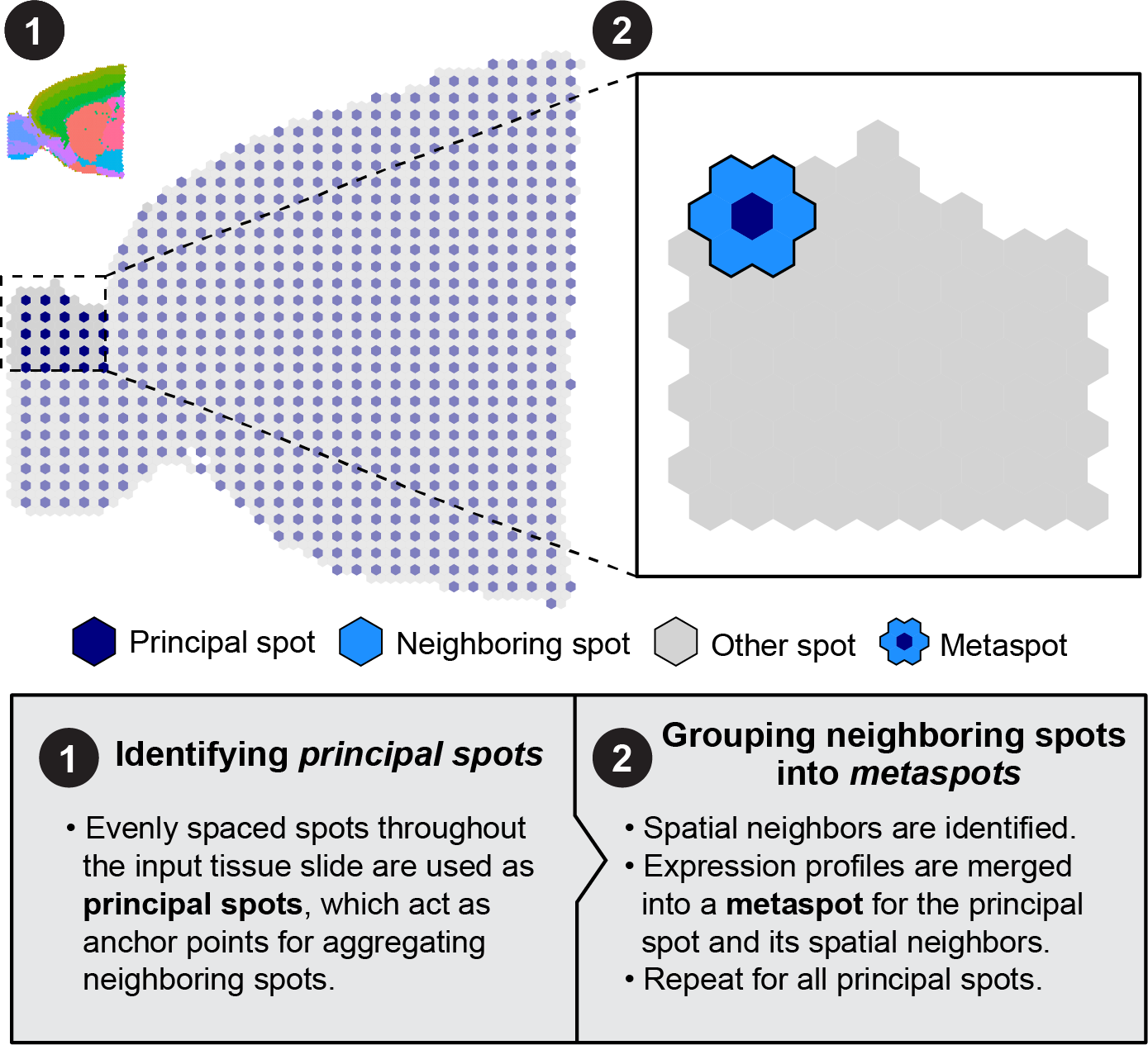
Visium ST generates sparse gene expression profiles in each spot,
thus introducing the same potential pitfalls as single-cell data for
co-expression network analysis. To alleviate these issues, hdWGCNA
includes a data aggregation approach to produce spatial
metaspots, similar to our metacell algorithm. This
approach aggregates neighboring spots based on spatial coordinates
rather than their transcriptomes. This procedure is performed in hdWGCNA
using the MetaspotsByGroups function.
Here we set up the data for hdWGCNA and
runMetaspotsByGroups. Similar to
MetacellsByGroups, the group.by parameter
slices the Seurat seurat_vhd to construct metaspots separately for each
group. Here we are just grouping by the ST slides to perform this step
separately for the anterior and posterior sample, but you could specify
cluster or anatomical regions as well to suit your analysis.
seurat_obj <- SetupForWGCNA(
  seurat_obj,
  gene_select = "fraction",
  fraction = 0.05,
  wgcna_name = "vis"
)

seurat_obj <- MetaspotsByGroups(
  seurat_obj,
  group.by = c("region"),
  ident.group = "region",
  assay = 'Spatial'
)
seurat_obj  <- NormalizeMetacells(seurat_obj)
The metaspot seurat_vhd is used everywhere that the metacell
seurat_vhd would be used for downstream analysis. For example, to
extract the metaspot seurat_vhd, you can run the
GetMetacellseurat_vhd function.
m_obj <- GetMetacellseurat_vhd(seurat_obj)
m_obj
An seurat_vhd of class Seurat
31053 features across 1505 samples within 1 assay
Active assay: Spatial (31053 features, 0 variable features)Co-expression network analysis
Now we are ready to perform co-expression network analysis using an identical pipeline to the single-cell workflow. For this analysis, we are performing brain-wide network analysis using all spots from all regions, but this analysis could be adjusted to perform network analysis on specific regions.
# set up the expression matrix, set group.by and group_name to NULL to include all spots
seurat_obj  <- SetDatExpr(
  seurat_obj,
  group.by=NULL,
  group_name = NULL
)

# test different soft power thresholds
seurat_obj <- TestSoftPowers(seurat_obj)
plot_list <- PlotSoftPowers(seurat_obj)

wrap_plots(plot_list, ncol=2)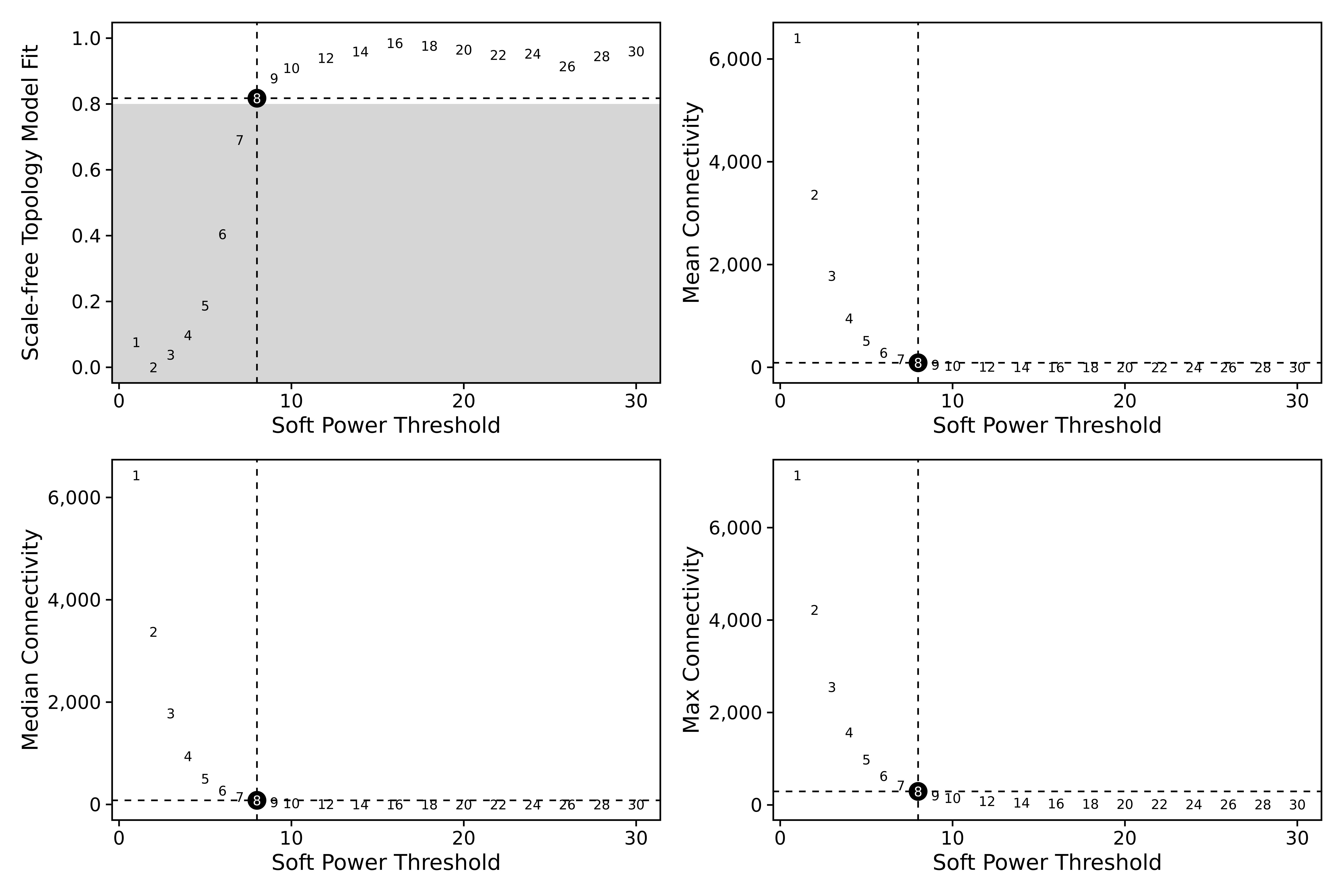
# construct co-expression network:
seurat_obj <- ConstructNetwork(
  seurat_obj,
  tom_name='test',
  overwrite_tom=TRUE
)

# plot the dendrogram
PlotDendrogram(seurat_obj, main='Spatial hdWGCNA dendrogram')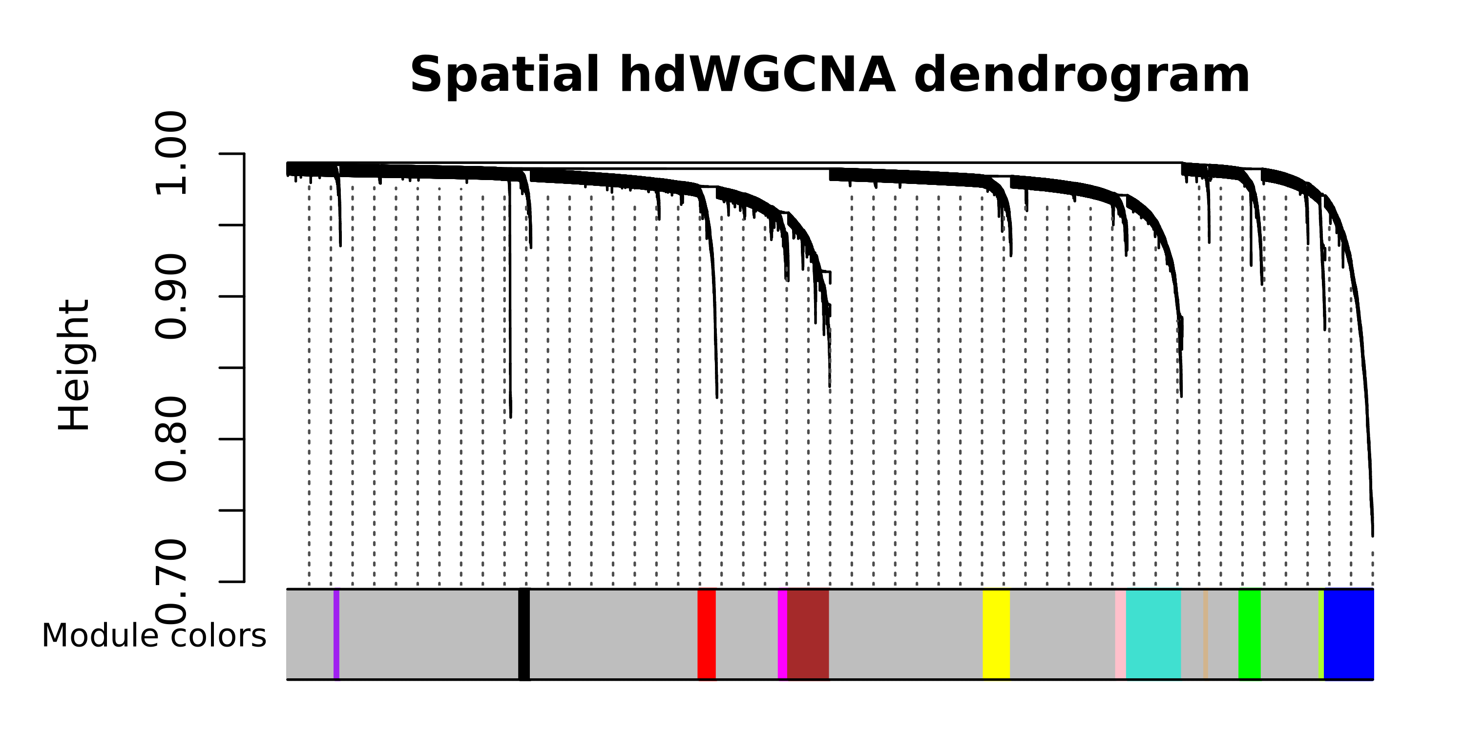
Next, we compute module eigengenes (MEs) and eigengene-based
connectivities (kMEs) using the ModuleEigengenes and
ModuleConnectivity functions respectively.
seurat_obj <- ModuleEigengenes(seurat_obj)
seurat_obj <- ModuleConnectivity(seurat_obj)
Here we reset the module names with the prefix “SM” (spatial modules). This step is optional.
seurat_obj <- ResetModuleNames(
  seurat_obj,
  new_name = "SM"
)
Data visualization
Here we visualize module eigengenes using the Seurat functions
DotPlot and SpatialFeaturePlot. For network
visualization, please refer to the Network visualization
tutorial.
# get module eigengenes and gene-module assignment tables
MEs <- GetMEs(seurat_obj)
modules <- GetModules(seurat_obj)
mods <- levels(modules$module); mods <- mods[mods != 'grey']

# add the MEs to the seurat metadata so we can plot it with Seurat functions
seurat_obj@meta.data <- cbind(seurat_obj@meta.data, MEs)

# plot with Seurat's DotPlot function
p <- DotPlot(seurat_obj, features=mods, group.by = 'annotation', dot.min=0.1)

# flip the x/y axes, rotate the axis labels, and change color scheme:
p <- p +
  coord_flip() +
  RotatedAxis() +
  scale_color_gradient2(high='red', mid='grey95', low='blue') +
  xlab('') + ylab('')

p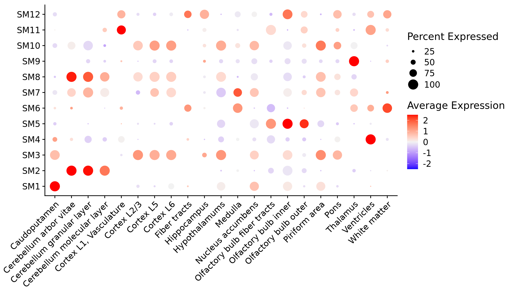
We can visualize the MEs directly on the spatial coordinates using
SpatialFeaturePlot.
p <- SpatialFeaturePlot(
  seurat_obj,
  features = mods,
  alpha = c(0.1, 1),
  ncol = 8
)

p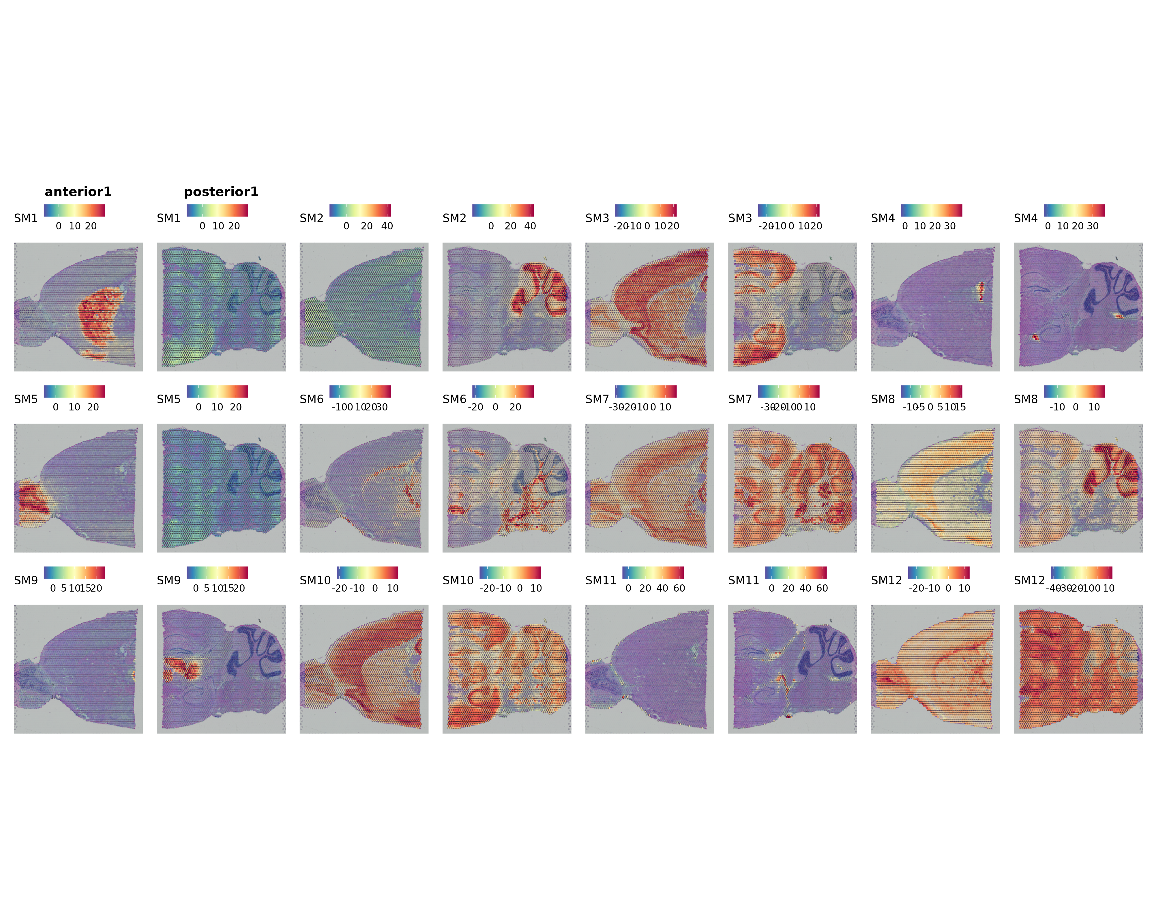
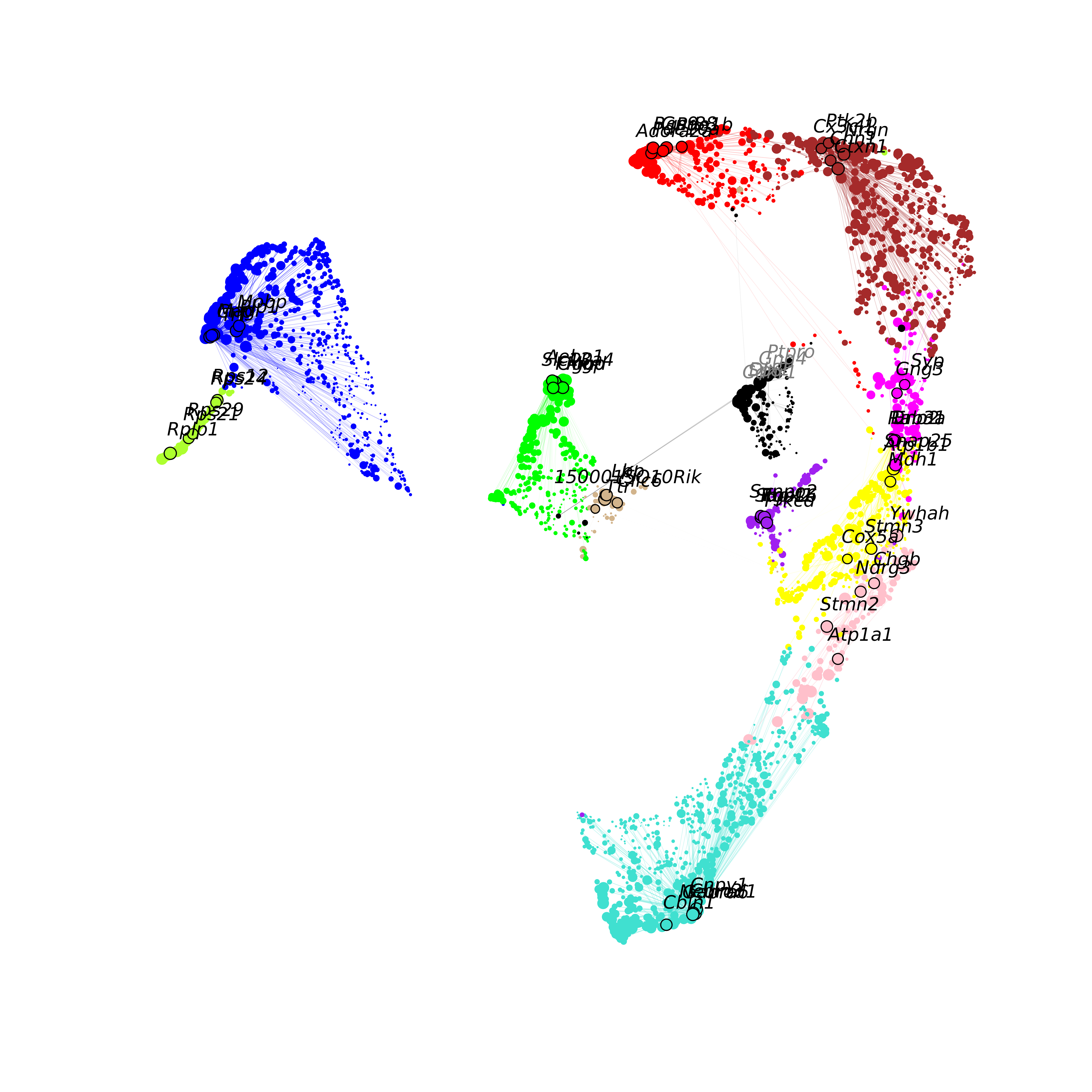
Next we visualize the co-expression network using UMAP. Please refer to the network visualization tutorial for more details about visualizing the co-expression network.
# perform UMAP embedding on the co-expression network
seurat_obj <- RunModuleUMAP(
  seurat_obj,
  n_hubs = 5,
  n_neighbors=15,
  min_dist=0.3,
  spread=1
)

# make the network plot
ModuleUMAPPlot(
  seurat_obj,
  edge.alpha=0.5,
  sample_edges=TRUE,
  keep_grey_edges=FALSE,
  edge_prop=0.075,
  label_hubs=5
)
Curio Seeker Dataset
In this section we perform a similar analysis using a mouse hippocampus dataset from Curio Bioscience. This dataset is not publicly available, but we obtained this dataset directly from Curio by filling out this form on their website. Curio provided a fully processed Seurat seurat_vhd, so for this tutorial we are simply using the Seurat seurat_vhd and clustering that they provided.
Load dataset
First we load the Seurat seurat_vhd containing the mouse hippocampus dataset provided by Curio. We will also make a few plots to show the clustering in transcriptome space (UMAP reduction) and in the biological coordinates. Note that this dataset provides a “dim reduction” called “SPATIAL” which contains the 2D biological coordinates.
# load the Seurat seurat_vhd
seurat_curio <- readRDS(paste0(data_dir, 'curio_datasets/Mouse_hippocampus_v1pt1/Mouse_hippocampus_seurat.rds'))

# make a dimplot in transcriptome space
p1 <- DimPlot(seurat_curio, label=TRUE, reduction = "umap") +
  NoLegend() + umap_theme() + ggtitle('UMAP')

# make a dimplot in biological space
p2 <- DimPlot(seurat_curio, reduction='SPATIAL', pt.size=0.5) +
  umap_theme() + ggtitle('Spatial')

p1 | p2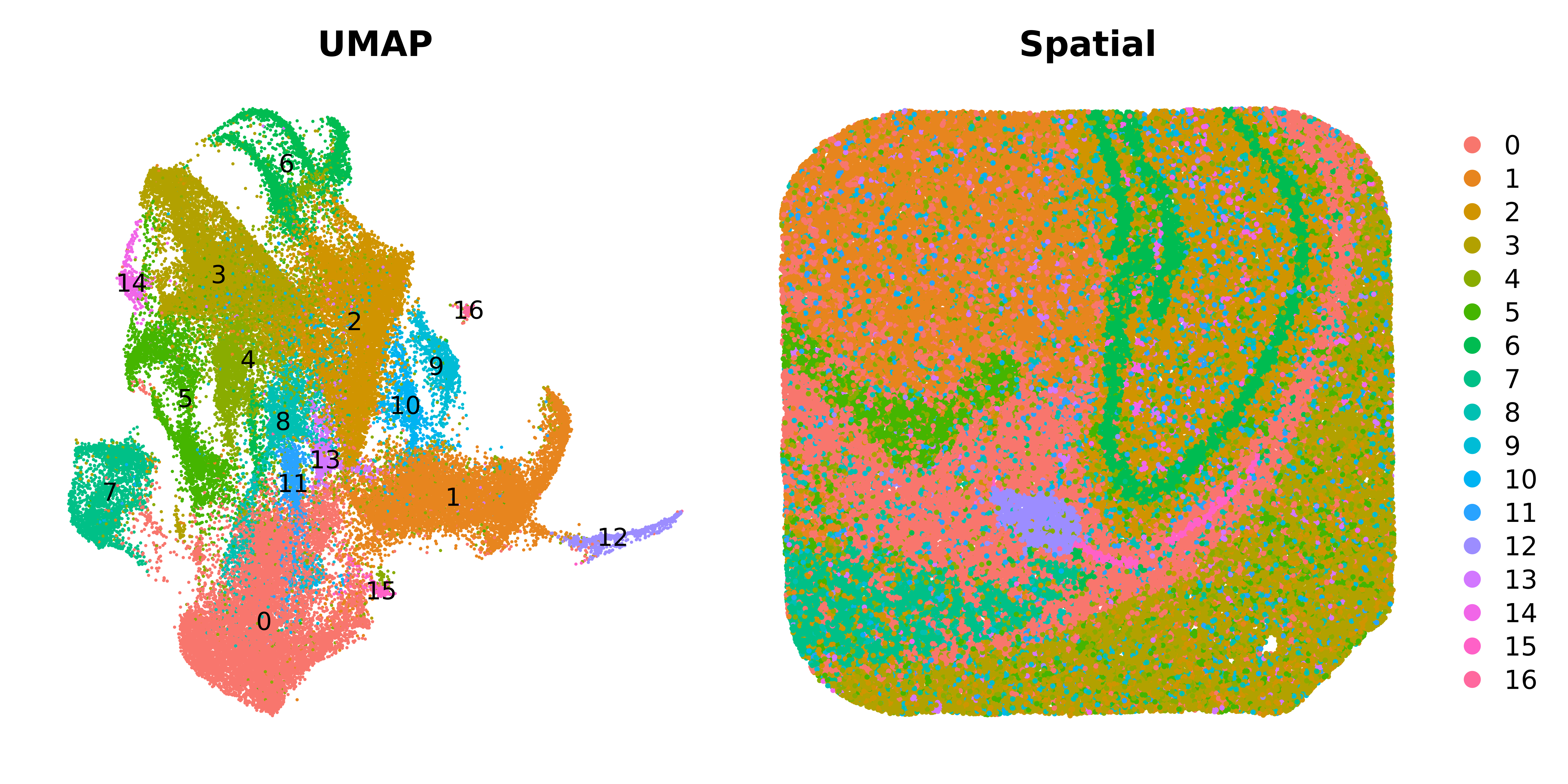
This plot is a little crowded so can make another
DimPlot split by cluster to see each
cluster on its own.
p <- DimPlot(
  seurat_curio,
  split.by='seurat_clusters',
  reduction = 'SPATIAL',
  ncol=6
) + NoLegend() + umap_theme()

p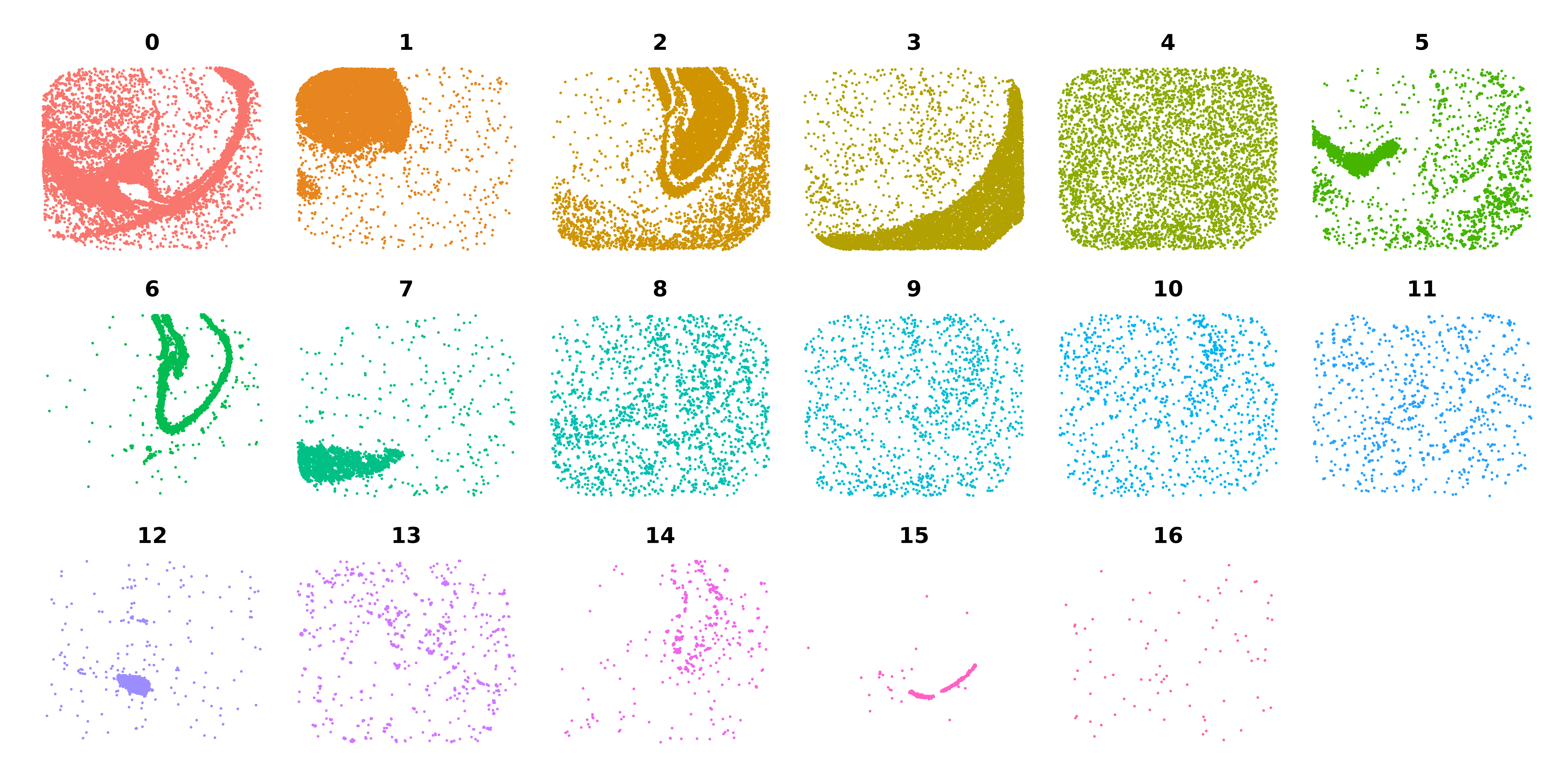
Construct Metacells with MetacellsByGroups
While Visium ST uses a grid of spots to assign molecular barcodes in
space, Curio Seeker uses small beads to capture transcriptome
information at 10 microns. Importantly, these beads are not regularly
spaced like in Visium. Therefore, the MetaspotsByGroups
function that we used for the Visium dataset is not appropriate for
Curio Seeker data. Instead, we will use MetacellsByGroups
but we will specify the reduction as the spatial
information, so cells that are close together in biological space will
be aggregated into metacells.
# Change the default assay to "RNA", SCTransform is generally not recommended for hdWGCNA.
seurat_curio <- DefaultAssay(seurat_curio, 'RNA')

seurat_curio <- SetupForWGCNA(
  seurat_curio,
  gene_select = "fraction",
  fraction = 0.01,
  wgcna_name = "curio"
)

# construct metacells  in each group
seurat_curio <- MetacellsByGroups(
  seurat_obj = seurat_curio,
  group.by = c("seurat_clusters"),
  ident.group = 'seurat_clusters',
  reduction = 'SPATIAL',
  k = 50,
  max_shared = 15,
  assay = 'RNA'
)

# normalize metacell expression matrix:
seurat_curio <- NormalizeMetacells(seurat_curio)
We can calculate the average X and Y coordinates for each metacell and plot them to check if they are aggregated based on spatial proximityfor each cluster as we expect.
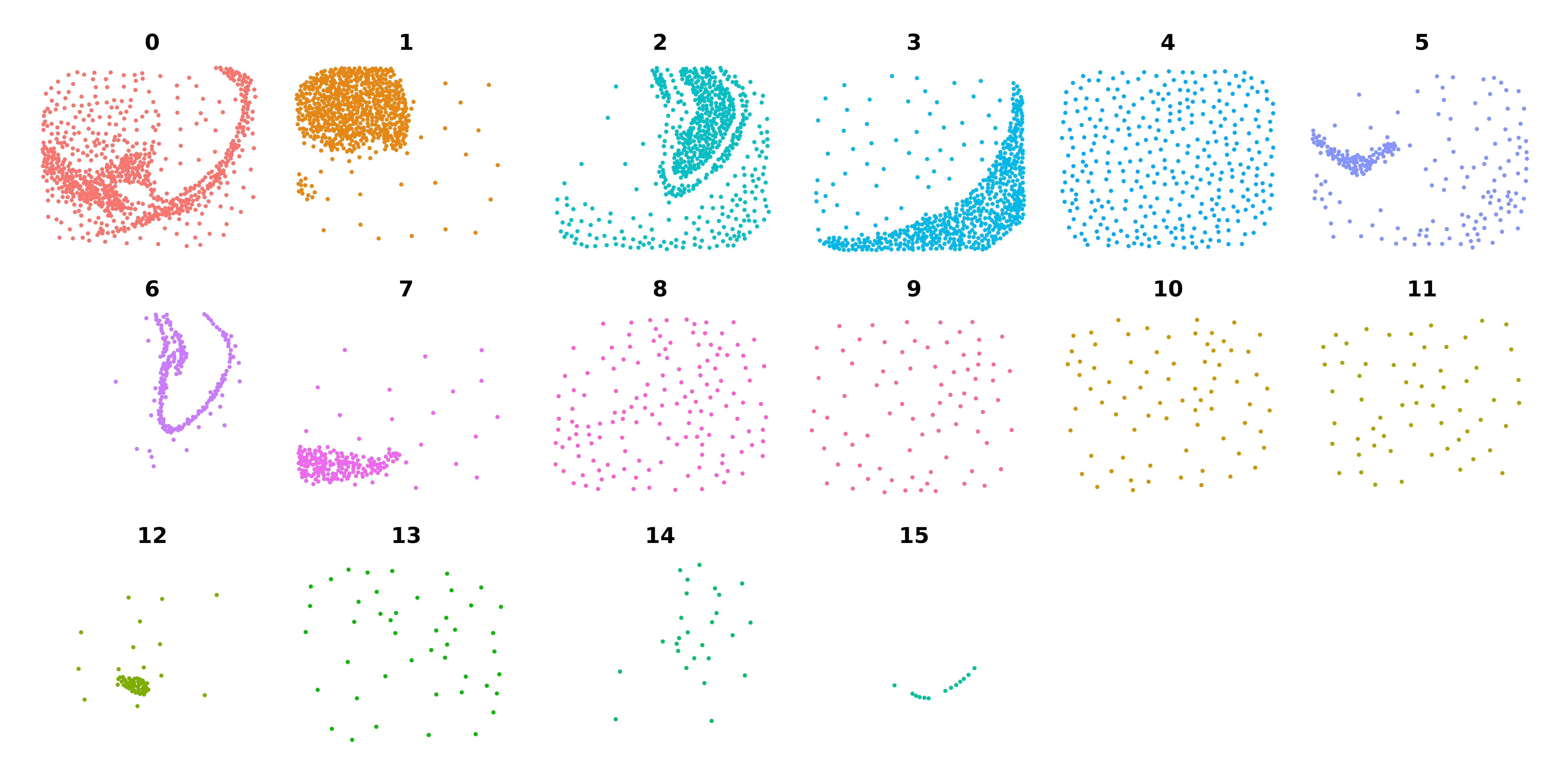
Show code for calculating metacell spatial coordinates
# get the metacell seurat_vhd
m_obj <- GetMetacellseurat_vhd(seurat_curio)
m_obj$seurat_clusters <- factor(
  m_obj$seurat_clusters,
  levels = levels(seurat_curio$seurat_clusters)
)

# get the image coordinates from the seurat obj and add to the metadata
spatial_coords <- seurat_curio@images$slice1@coordinates
seurat_curio@meta.data$spatial_x <- spatial_coords$x * -1
seurat_curio@meta.data$spatial_y <- spatial_coords$y
seurat_curio$barcode <- colnames(seurat_curio)

# loop over each metacell and calculate the average X and Y
meta_spatial_coords <- do.call(rbind, lapply(1:ncol(m_obj), function(i){
  x <- m_obj@meta.data$cells_merged[i]
  cur_bcs <- str_split(x, ',')[[1]]
  cur_df <- subset(seurat_curio@meta.data, barcode %in% cur_bcs)
  cur_x <- mean(cur_df$spatial_x)
  cur_y <- mean(cur_df$spatial_y)
  data.frame(spatial_1 = cur_y, spatial_2=cur_x)
}))
rownames(meta_spatial_coords) <- colnames(m_obj)

# add this as a dim reduct
m_obj@reductions$spatial <- CreateDimReducseurat_vhd(
  embeddings = as.matrix(meta_spatial_coords),
  key = 'spatial'
)

p <- DimPlot(
  m_obj,
  split.by='seurat_clusters',
  reduction = 'spatial',
  ncol=6
) + NoLegend() + umap_theme()

p
Co-expression network analysis
Now that we have our metacells, we next carry out co-expression network analysis with hdWGCNA, similar to as we have done before. Here we perform network analysis on cluster 6, which appears to contain the pyramidal layer of the hippocampus and the granular layer of the dentate gyrus.
# set up the expression matrix
seurat_curio  <- SetDatExpr(
  seurat_curio,
  group.by='seurat_clusters',
  group_name = '6'
)

# test different soft power thresholds
seurat_curio <- TestSoftPowers(seurat_curio)

# construct co-expression network:
seurat_curio <- ConstructNetwork(
  seurat_curio,
  tom_name='curio',
  overwrite_tom=TRUE
)

# compute module eigengenes & connectivity
seurat_curio <- ModuleEigengenes(seurat_curio)
seurat_curio <- ModuleConnectivity(
  seurat_curio,
  group.by = 'seurat_clusters',
  group_name = '6'
)

# plot the dendrogram
PlotDendrogram(seurat_curio, main='Curio hdWGCNA dendrogram')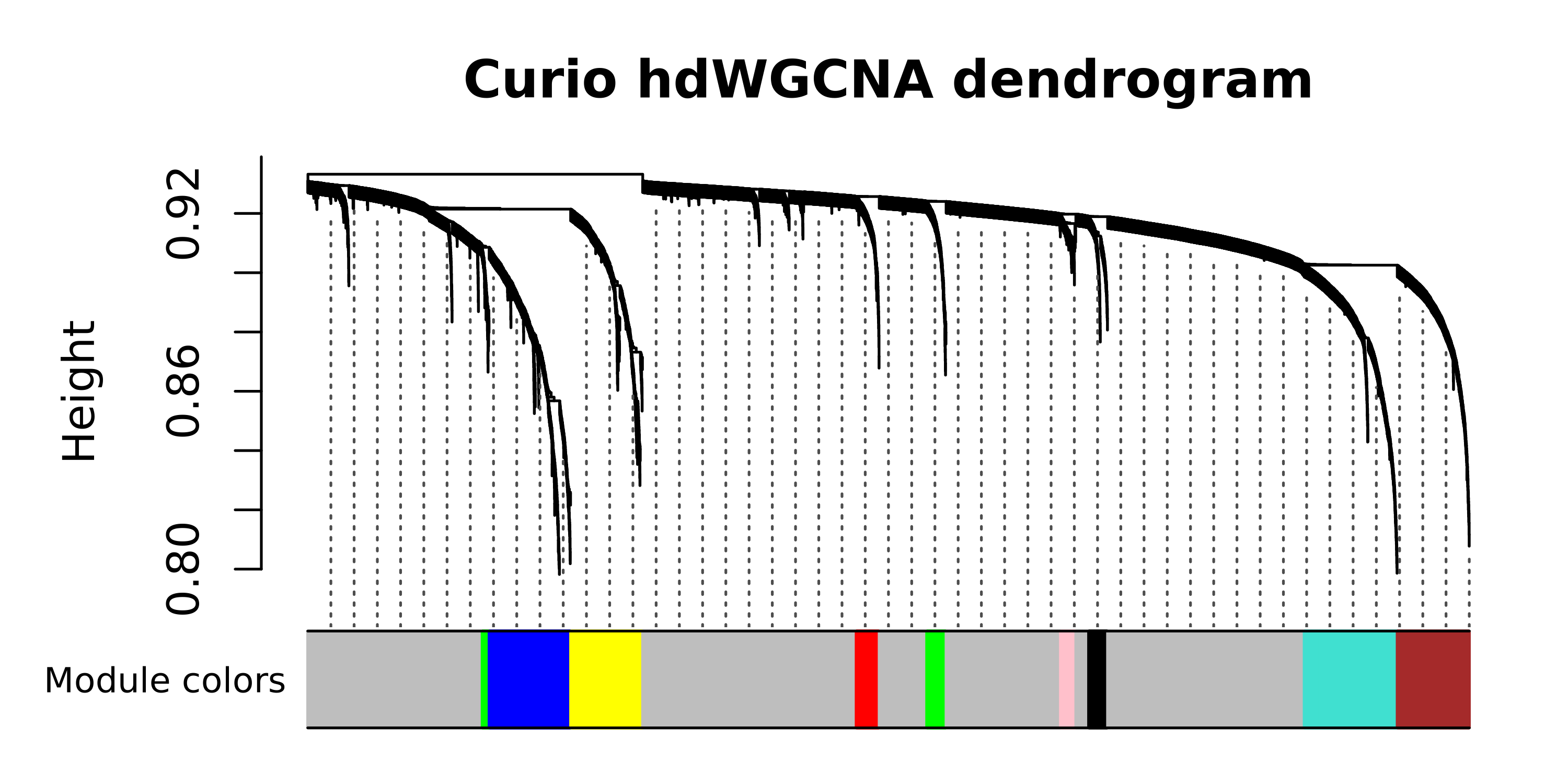
Next we plot the expression of these modules in the tissue coordinates.
plot_list <- ModuleFeaturePlot(
  seurat_curio,
  reduction = 'SPATIAL',
  restrict_range=FALSE
)

wrap_plots(plot_list, ncol=4)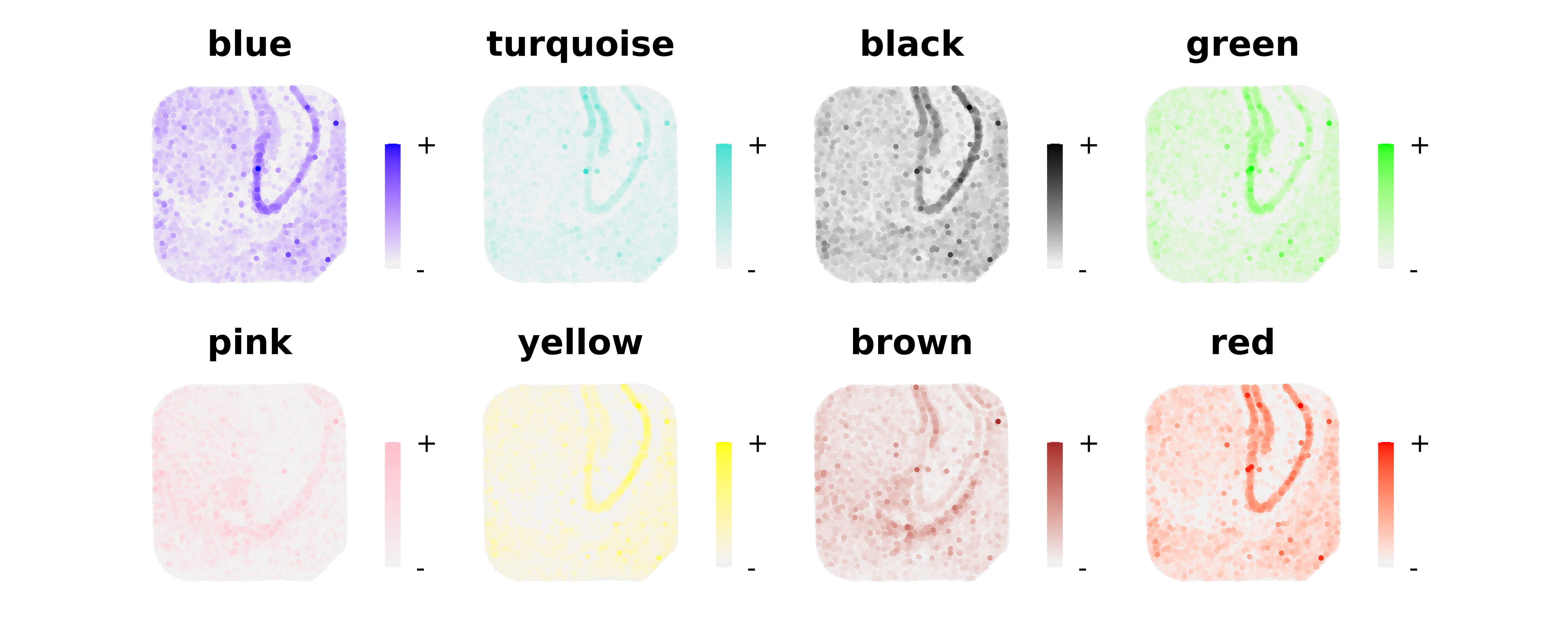
This concludes the part of the tutorial for the Curio dataset, but from here we could proceed to perform downstream analysis and more data visualization.
10X Visium HD Dataset
Here we perform a similar analysis using Visium HD, the second major version of sequencing-based ST from 10X Genomics. This is a similar technology to the standard Visium, where the main difference is that the “spots” are much smaller and there is no gap in between them. Visium HD spots are closer to single-cell resolution, however some spots may still span more than one cell, and furthermore one spot could be subcellular.
Overall, this workflow is similar to the one shown for the Curio Seeker dataset.
Load dataset
The mouse brain Visium HD dataset can be downloaded diectly from 10X Genomics at this link.
# use the 008um resolution for this tutorial
seurat_vhd <- Load10X_Spatial(data.dir='path/to/dataset/square_008um/')
Clustering analysis
Here we follow the Seurat Visium HD tutorial to perform a basic clustering analysis. In practice, you should perform clustering analysis and QC that best suits your dataset, here we simply use Seurat for convenience to demonstrate hdWGCNA.
seurat_vhd <- NormalizeData(seurat_vhd)
seurat_vhd <- FindVariableFeatures(seurat_vhd)
seurat_vhd <- ScaleData(seurat_vhd)
seurat_vhd <- RunPCA(seurat_vhd)
seurat_vhd <- FindNeighbors(seurat_vhd, reduction = "pca", dims = 1:30)
seurat_vhd <- FindClusters(seurat_vhd)

# get the image coordinates from the seurat obj and add to the metadata
spatial_coords <- as.data.frame(seurat_vhd@reductions$spatial@cell.embeddings)
seurat_vhd@meta.data$spatial_x <- spatial_coords$spatial_1 * -1
seurat_vhd@meta.data$spatial_y <- spatial_coords$spatial_2
seurat_vhd$barcode <- colnames(seurat_vhd)

# add this as a dim reduct
seurat_vhd@reductions$spatial <- CreateDimReducObject(
  embeddings = as.matrix(spatial_coords),
  key = 'spatial'
)

p <- DimPlot(
  seurat_vhd,
  split.by='seurat_clusters',
  reduction = 'spatial',
  ncol=9
) + NoLegend() + umap_theme()

p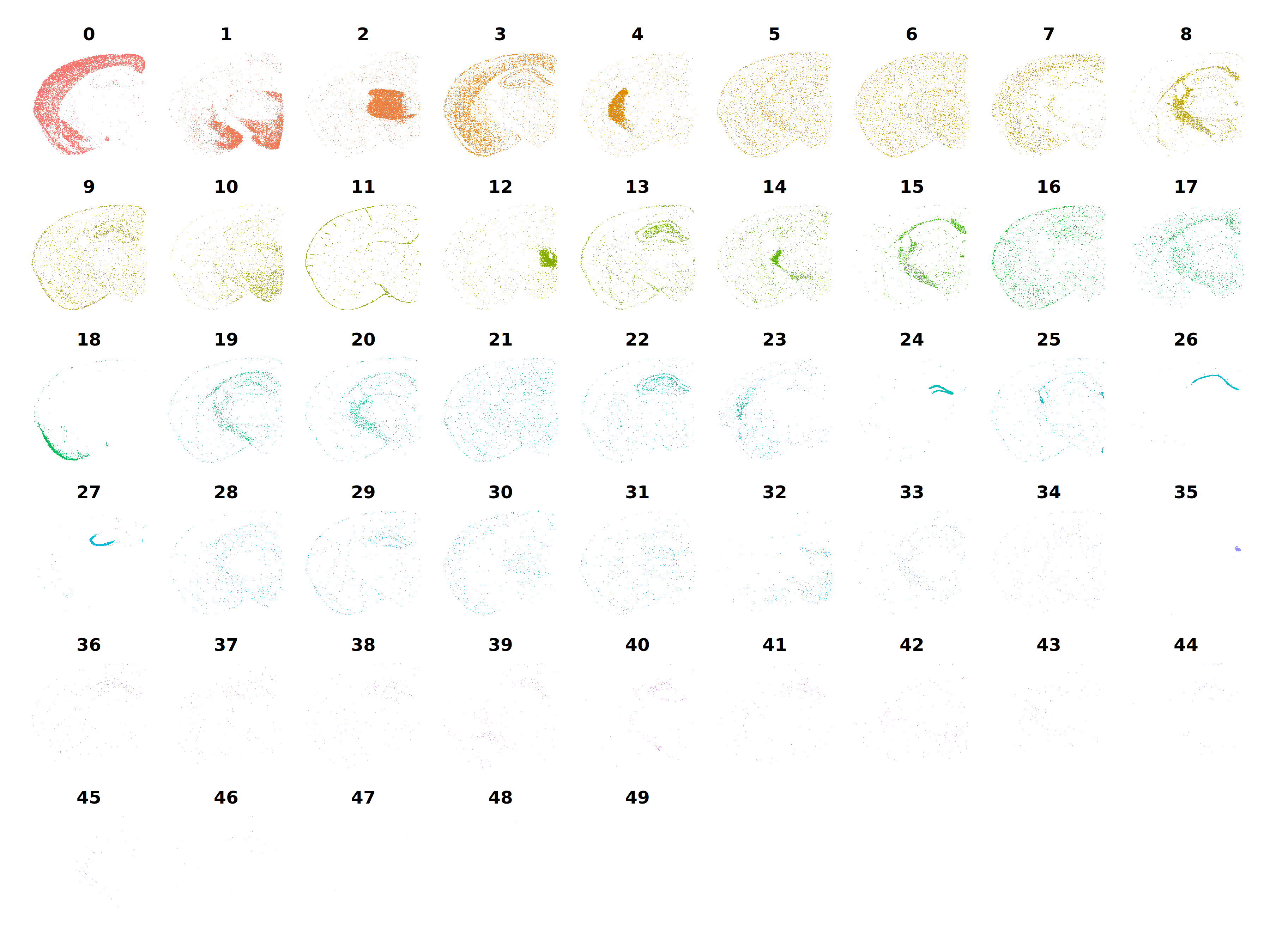
Construct Metacells with MetacellsByGroups
Here we set up the genes that we will use for co-expression network
analysis (variable features), and then we construct metacells. For
Visium HD, we will merge spatially proximal spots using the
MetacellsByGroups function instead of
MetaspotsByGroups, which is only used for standard Visium.
In order for us to use MetacellsByGroups for spatial data,
similar to the Curio dataset, we need to create a “dimensionality
reduction” in the Seurat object that contains the spatial
coordinates.
# create the spatial reduction
coords <- as.matrix(GetTissueCoordinates(seurat_vhd)[,c('x', 'y')])
colnames(coords) <- c('spatial_1', 'spatial_2')
seurat_vhd@reductions$spatial <- CreateDimReducObject(
embeddings = coords,
assay = 'RNA',
key = 'spatial_'
)
seurat_vhd <- SetupForWGCNA(
seurat_vhd,
gene_select = "variable",
wgcna_name = "vhd"
)
length(GetWGCNAGenes(seurat_vhd))
# construct metacells in each group
seurat_vhd <- MetacellsByGroups(
seurat_obj = seurat_vhd,
group.by = c("seurat_clusters"),
ident.group = 'seurat_clusters',
reduction = 'spatial',
k = 50,
max_shared = 15
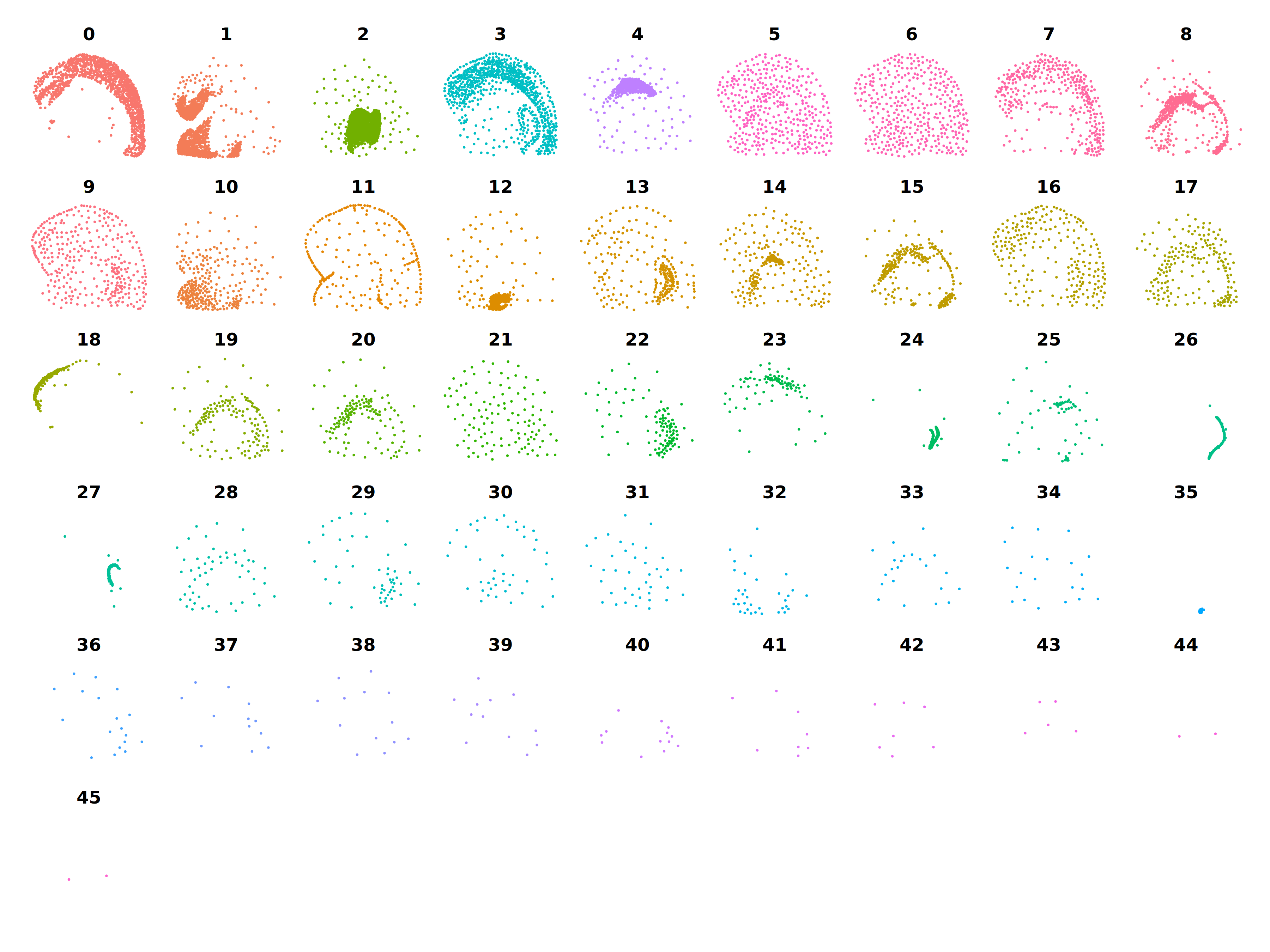
)We can calculate the average X and Y coordinates for each metacell and plot them to check if they are aggregated based on spatial proximityfor each cluster as we expect.
Show code for calculating metacell spatial coordinates
# get the metacell object
m_obj <- GetMetacellObject(seurat_vhd)
m_obj$seurat_clusters <- factor(
  m_obj$seurat_clusters,
  levels = levels(seurat_vhd$seurat_clusters)
)

# get the image coordinates from the seurat obj and add to the metadata
spatial_coords <- as.data.frame(seurat_vhd@reductions$spatial@cell.embeddings)
seurat_vhd@meta.data$spatial_x <- spatial_coords$spatial_1 * -1
seurat_vhd@meta.data$spatial_y <- spatial_coords$spatial_2
seurat_vhd$barcode <- colnames(seurat_vhd)

# loop over each metacell and calculate the average X and Y
meta_spatial_coords <- do.call(rbind, lapply(1:ncol(m_obj), function(i){
  x <- m_obj@meta.data$cells_merged[i]
  cur_bcs <- str_split(x, ',')[[1]]
  cur_df <- subset(seurat_vhd@meta.data, barcode %in% cur_bcs)
  cur_x <- mean(cur_df$spatial_x)
  cur_y <- mean(cur_df$spatial_y)
  data.frame(spatial_1 = cur_y, spatial_2=cur_x)
}))
rownames(meta_spatial_coords) <- colnames(m_obj)

# add this as a dim reduct
m_obj@reductions$spatial <- CreateDimReducObject(
  embeddings = as.matrix(meta_spatial_coords),
  key = 'spatial'
)

p <- DimPlot(
  m_obj,
  split.by='seurat_clusters',
  reduction = 'spatial',
  ncol=9
) + NoLegend() + umap_theme()

p
Co-expression network analysis
We are now ready to perform co-expression network analysis, similar to as we did above.
# set up the expression matrix
seurat_vhd  <- SetDatExpr(seurat_vhd)

# test different soft power thresholds
seurat_vhd <- TestSoftPowers(seurat_vhd)

# construct co-expression network:
seurat_vhd <- ConstructNetwork(
  seurat_vhd,
  tom_name='vhd'
)

# compute module eigengenes & connectivity
seurat_vhd <- ModuleEigengenes(seurat_vhd)
seurat_vhd <- ModuleConnectivity(
  seurat_vhd
)

# plot the dendrogram
PlotDendrogram(seurat_vhd, main='Visium HD hdWGCNA dendrogram')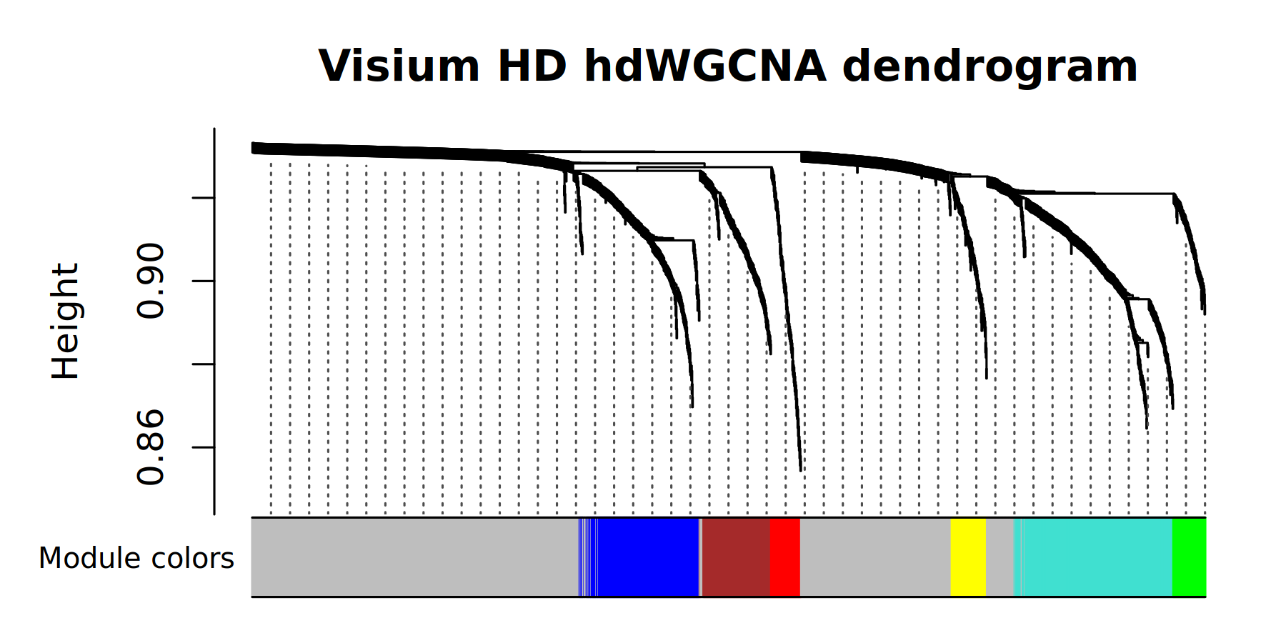
Next we plot the expression of these modules in the spatial coordinates.
plot_list <- ModuleFeaturePlot(
  seurat_vhd,
  reduction = 'spatial',
  restrict_range=FALSE
)

wrap_plots(plot_list, ncol=3)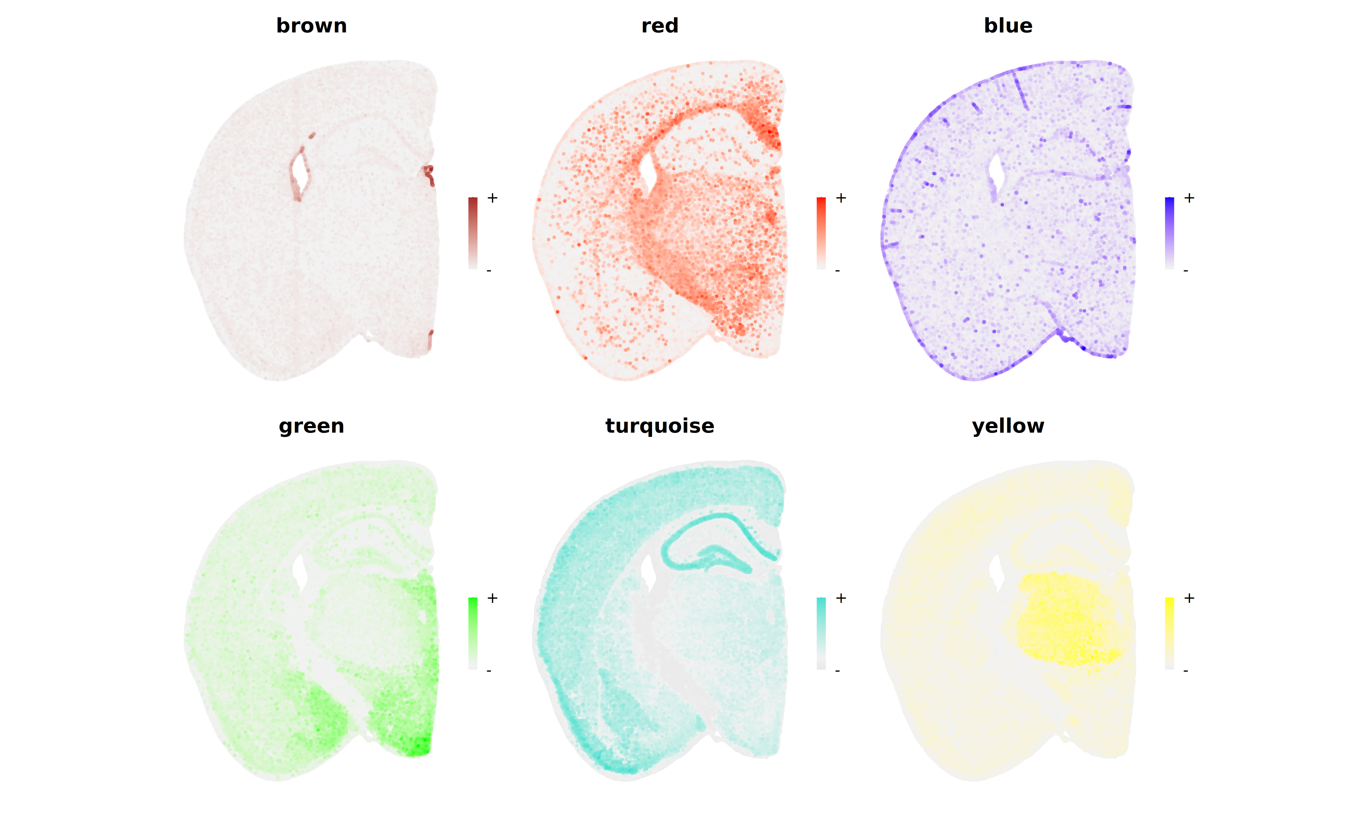
This concludes the part of the tutorial for the Visium HD dataset, but from here we could proceed to perform downstream analysis and more data visualization.
Conclusion and next steps
In this tutorial we demonstrated the core functions for performing co-expression network analysis in two types of ST datasets: Visium and Slide-Seq. Now that you have constructed a co-expression network and identified gene modules, there are many downstream analysis tasks which you can take advantage of within hdWGCNA. To provide more depth to your co-expression modules, we encourage you to explore the network visualization tutorial and the enrichment analysis tutorial.
To compare different biological conditions using hdWGCNA, check out the following tutorials.
- Differential module eigengene (DME) tutorial
- Module preservation tutorial
- Module-trait correlation tutorial
For more advanced analysis, such as Transcription factor regulatory network analysis, please check out the following tutorials.